Complex Time Series VI, recurrence plots
To conclude this series on complex time series and their characterization using graphical tools I will show you a tool called recurrence plot, which allows to obtain some measures used in the recurrence quantification analysis, or RQA for its acronym in English. The recurrence is a characteristic property of deterministic dynamical systems, and consists of that two or more states of the system are arbitrarily close after a certain period of time.
As usual, if you want to start the series at the beginning, this is the link to the first article of the series on graphic characterization of complex time series. In this other link you can download the executable and source code of the GraphStudy project, written in CSharp with Visual Studio 2013.
The recurrence plots are a graphical tool whose interpretation requires experience, so that, in a post of a blog I cannot delve too deeply into the subject. For more information on this subject, in this link you have a website entirely devoted to recurrent plots, and in this other you have a book about recurrence quantification analysis.
In the previous article I showed how to extend the phase space from one dimension to two or three dimensions, to try to reconstruct approximately the attractor of the system. With recurrence plots the idea is similar, it consists to obtain a number of points with a dimension greater or equal of two, using the series values displaced a fixed period of time to build them. But in recurrence plots we are not limited to a three-dimensional space at most, as they are always represented in two dimensions, regardless of the dimension we have chosen to study the recurrence of the series.
Once obtained a number N of points Xi with dimension m from the original series, each one with coordinates xi, xi+t, xi+2t,..., xi+(m-1)t, what we do is to draw a square matrix in which each Rij element represents the distance between the points Xi and Xj of the m-dimensional series. This matrix is symmetrical respect the main diagonal. When the distance between two points is below a certain threshold, we say that the system presents a recurrence.
This matrix can be represented in two ways, on one hand, each point can be represented by a different color whose intensity depends on the distance calculated for that position, or it can be represented in black, to indicate that in this position there is a recurrence, or in white otherwise.
Given the distribution of recurrence points in the recurrence plot, you can perform a quantification of that diagram, which involves making a series of measures that will allow us to characterize the dynamics of the system.
Recurrence plots in GraphStudy
In the GraphStudy application you can get recurrence plots by opening a csv or tsd file, and using the L. Extend or P. Extend options as we saw in the previous article on the study of the autocorrelation in the series. As I showed there, we must first calculate the autocorrelation in the series and then select a distance greater than zero by clicking the right mouse button over the graph of correlation. Then you must select the R. Plot tab:
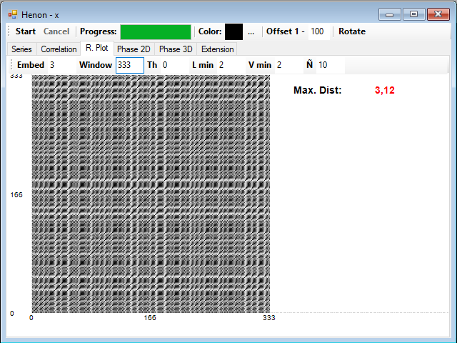
The first parameters you have to know are Embed, representing the embedded dimension m, i.e., the dimension to which we are extending the series, Window, which is simply the width and height of the matrix, i.e., the number of points of the series that are used to build the graph. This number is limited by the amount of samples and the width and height of the window where the graph is shown. Finally, Th is the threshold of the distance below which it is considered that two points are a recurrence, this parameter is also called radius.
Typically, you can select a value Th approximately 10% of the maximum distance, which is shown next to the graph. If Th is zero, the graph is represented using a color scale. In GraphStudy a gray scale is used, using black for the minimum distance and white for the maximum.
If you change any of these parameters, you have to double-click on the graph to see the results. If a value other than zero is selected for Th, also the most common RQA measures are displayed next to the graph:
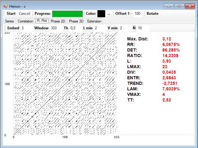
The distance that I use in the program is the Euclidean one, but it can easily be changed in the source code to a different one in the class that draws the map, which is RecurrenceMapDrawer.
As for the measures, the first is RR, recurrence rate, and is simply the percentage of recurrent points in the graph. In this program I'm not counting the points on the main diagonal (recurrence of a point with himself). This, and all other measures, depends, obviously, from the value selected for Th.
The study of the diagonal lines on the graph, gives us an idea of the degree of determinism and predictability of the series. These measures depend on the L min parameter, which indicates the minimum number of points that must have a diagonal line to be taken into account in these measures (the main diagonal is not taken into account in any case), and they are as follows:
- DET, or percentage of determinism, which is simply the percentage of recurrence points that are forming diagonal lines.
- L or average diagonal line is the average length of the diagonal lines.
- LMAX is the length of the longest diagonal line.
- DIV, or divergence, is the inverse of LMAX, and is related to the sum of positive Lyapunov exponents.
- RATIO, is the relationship between DET and RR.
- ENTR or Shannon entropy of the frequency distribution of the lengths of the diagonal lines, defined as
-Σp(l)log(p(l)), being p(l) the probability of finding a diagonal line of length l.
With vertical lines we obtain similar measures dependent of the V min parameter, which indicates the minimum size of these lines:
- LAM, or laminarity percentage, which is the rate of points forming vertical lines of recurrent points.
- VMAX, which is the maximum length of the vertical lines.
- TT, indicates the average length of the vertical lines.
Finally, related to the parameter Ñ is the TREND measure, this parameter Ñ represents a distance in diagonal lines from the main diagonal. The coefficient of linear regression of the density of points in diagonals parallel to the main diagonal until this distance is calculated, and gives us a measure of the stationarity of the dynamic system.
Here is an example of recurrence plot for a random series:
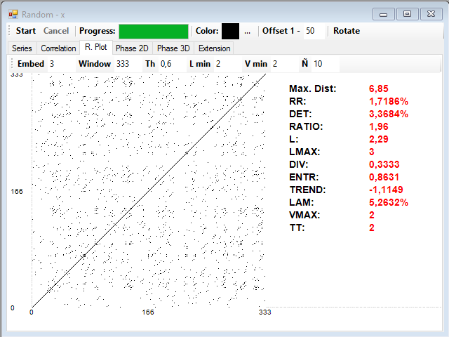
You can see that the DET measure is very low, the map is composed practically only of isolated points. However, a series from a sinusoidal signal has a completely different plot:
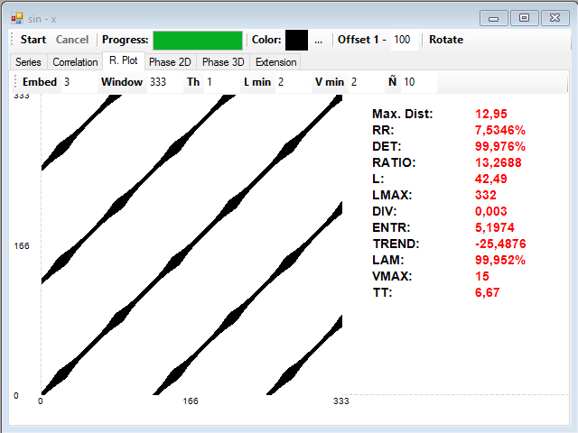
In any case, the interpretation of measures and work with recurrence plots require experience and some explanations that are beyond the possibilities of a simple post, so I recommend you to use the links above if you want to deepen the study of the topic.
Recurrence plots with R
With the R program you can do also recurrence plot analysis, there are several packages to draw the plots and obtain RQA measurements. As an example you can download the series with 1000 terms of the x variable of the Henon system.
You can load the time series with the following command:
rhen<-as.ts(read.csv("henon-x.csv",F))
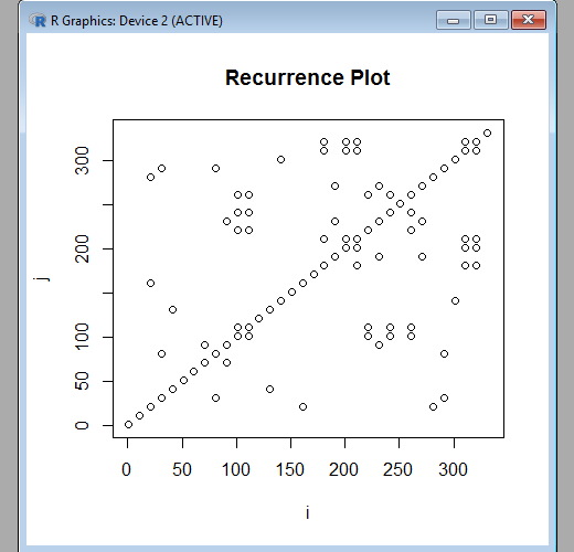
With the fNonlinear package you can draw a recurrence plot, although somewhat rudimentary, with the following command:
recurrencePlot(rhen,3,1,333,0.3)
The parameters are, in this order, the set of values, the embedded dimension, the time delay, the width of the window and the threshold or radius. The result is like this:
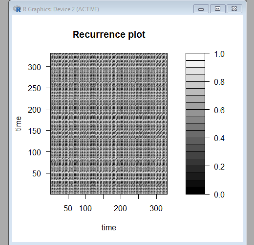
In the tseriesChaos package there is another function to draw a recurrence plot, using a gray scale:
recurr(rhen,3,1,0,333)
Where the parameters are, in order, the series of values, the embedded dimension, the time delay, the initial value and the final value of the window. The result is as follows:
For the RQA measures, we can use the crqa package, which also allows us to calculate measures for cross recurrence plots, in which two different series are compared instead of a single series with itself.
The function is as follows:
rqa<-crqa(rhen,rhen,delay=1,embed=3,radius=0.3,normalize=0,
          rescale=0,mindiagline=2,minvertline=2,side="lower")
The first two parameters are the set of values, this function is designed to compare two different series, to calculate cross-recurrence measures, but we can also get the measures for a single series in this way.
Next we have the time delay (delay) and embedded dimension (embed), the threshold or radius (radius), a value to indicate the type of normalization to perform (normalize), which we pass to zero to take no action, a value of re scaling (rescale) we give zero also to take no action, the minimum values for the diagonal and vertical lines (mindiagline and minvertline) and the side parameter, to indicate that part of the matrix that should be taken into account for calculations. With lower we indicate the lower triangle, with both the entire matrix is considered, including the main diagonal in the calculations.
Those are the calculated measures:
summary(rqa)
       Length Class     Mode
RR          1 -none-    numeric
DET         1 -none-    numeric
NRLINE      1 -none-    numeric
maxL        1 -none-    numeric
L           1 -none-    numeric
ENTR        1 -none-    numeric
rENTR       1 -none-    numeric
LAM         1 -none-    numeric
TT          1 -none-    numeric
NRLINE is the total number of lines on the plot, rENTR is the entropy normalized by the number of lines on the plot and the rest are the same I mentioned above.
I think that the RR measure is half of the real value, which may be due to a function error when calculating using only half of the matrix; it may divide by the total number of points, rather than by the number of points of that half.


