Complex Time Series V, autocorrelation and extended dimension
In this new article in the series on time series with complex dynamics, I will show you a procedure to approximately reconstruct the information of a dynamic system with two or more variables from a single series, i.e. a set of data in a single dimension. What we will get from this unique series is a new one for each of the extra dimensions with which we intend to extend the model.
As usual, if you want to start the series at the beginning, this is the link to the first article of the series on graphic characterization of complex time series. In this other link you can download the executable and source code of the GraphStudy project, written in CSharp with Visual Studio 2013.
The idea on which are based the reconstruction of new dimensions from the one-dimensional series is as follows: we assume that the series of values which we have corresponds to a variable of a dynamic system with more variables and, therefore, it contains information about the remaining variables (dimensions) of the system, since they all interact.
Based on the Whitney theorem of algebraic topology, we consider that we can reconstruct an attractor of the system that, though is not the same as the original system, it is topologically equivalent, and retains a similar structure and properties. To do this, we build another D-dimensional set of points, where D is the number of dimensions to which we want to extend the series, taking each of these dimensions a point of the original series, taken from a given position, displaced t elements from the position of the value in the previous dimension.
For example, to reconstruct in a three-dimensional space, we would take for each point, the values Xi, Xi+t and Xi+2t of the series, which would transform the Xi point, in one dimension, in the X3i three-dimensional one. With these points, we can draw the phase diagram and display the three-dimensional aspect of the supposed reconstructed attractor.
Note that not all series will allow us to reconstruct an attractor with more dimensions. It is possible, for example, that the series not contain information on other dimensions, or that they do not exist. It is an analysis tool that allows us to study whether the dynamic system from which comes the time series is chaotic and presents an attractor in two or more dimensions, not a magic recipe.
Autocorrelation and mutual information
The choice of the amount of the displacement t is determinant in the accuracy of the reconstructed attractor. To select an appropriate value, we can help us with the study of the correlation of the values in the series with those displaced t elements forward of them.
We can use the autocorrelation function, which is simply the linear correlation between the values of the series with an interval of d values of separation. With the GraphStudy application we can graph the correlation of the series at different distances. To do this, you must open a csv or tsd file (the native file format of the application) with the Open option from the File menu. For example, the Lorenz.tsd file with the Lorenz attractor.

With the L. Extend button you can access the form whit which you can draw the graph of the linear correlation between the elements of the series at different distances. Ensure that you have selected the corresponding series to the X variable.
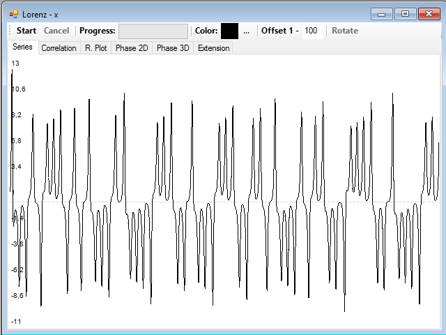
In the Offset text box you can define the maximum displacement you want to reach in the calculation of the correlation, the default is 100, which is more than enough in most cases, since at high distances the series no longer have practically autocorrelation, but, as this series is quite slow and it has 100000 values, you can select a greater distance, of 1000, for example.
To calculate the autocorrelation graph, simply click the Start button.
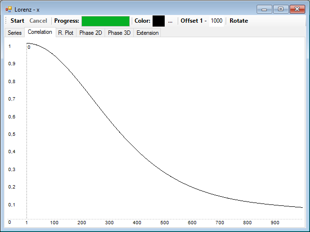
You can see that the correlation is slowly declining with distance.
The linear correlation provides information on linear relationships between sets of values, but this concept can be generalized to nonlinear relationships in nonlinear systems performing the calculation of the mutual information, based on the information theory.
For this all we need is a probability distribution of the values of the series separately and another for the different pairs of values at a given distance d. The joint information between the Xi and Xi+d elements of the series will be:
I(Xi,Xi+d) = log2[P(Xi,Xi+d)/(P(Xi)P(Xi+d))]
That is, the base-2 logarithm of the ratio between the probability (frequency) for the two values to appear at that distance and the product of the probabilities (frequencies) of the values separately.
If we extend this calculation to the entire series, for each distance d we have the mutual information of the series defined as:
I(d) = ΣP(Xi,Xi+d)I(Xi,Xi+d)
In GraphStudy, we can make this calculation similarly using the P. Extend button in the data panel, already used in the previous article in the series to obtain the frequency histogram of the values of the series:
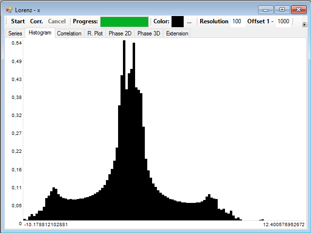
To calculate the histogram you have to press the Start button. Then the Corr button, to calculate and draw the mutual information of the series at different distances, whose range can also be changed in the Offset text box:
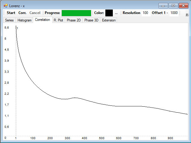
You can see that the mutual information also decreases rapidly with time.
Extending the dimension
Once you have the correlation graph, either of them, you can select on the distance to rebuild the attractor. First, you can see the original attractor using the 3D Phase button of the data panel, and the Rotate button to place it in a convenient perspective:
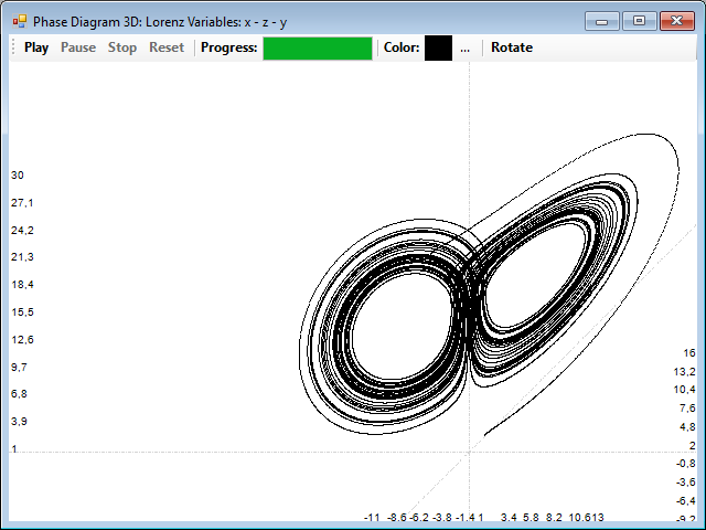
If you now click on one of the graphs of correlation with the left mouse button, a distance will be selected and you can see the corresponding attractor reconstructed in two dimensions, by selecting the Phase 2D tab, or three, selecting the Phase 3D tab. In this example, the distance is 22:
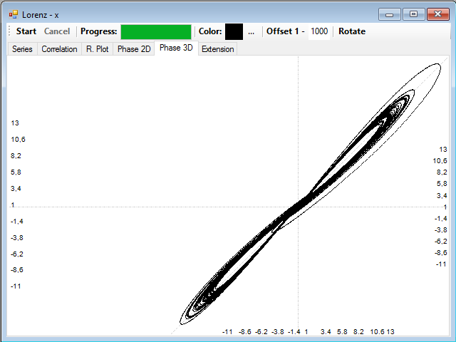
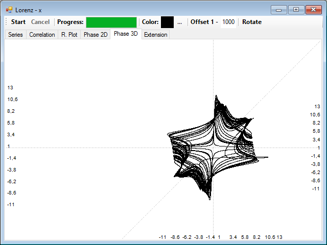
The correlation distance is too short and the attractor is highly compressed, if now you try a very long correlation distance, for example 500, the attractor is highly distorted because of the low correlation between the points:
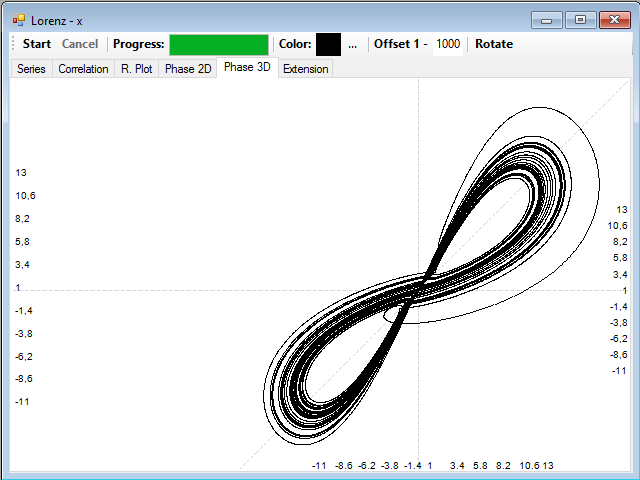
Selecting an intermediate value, for example about 100, we get a fairly good reconstruction of the entire attractor:
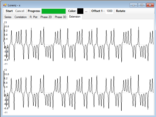
In the Extension tab are the displaced series for the other two variables Y and Z:
You can drag and drop one of them on a window showing the real series corresponding to the variable, in order to perform a visual comparison, for example, this is the reconstruction of the Y series (red) overlaid with the original one (black):
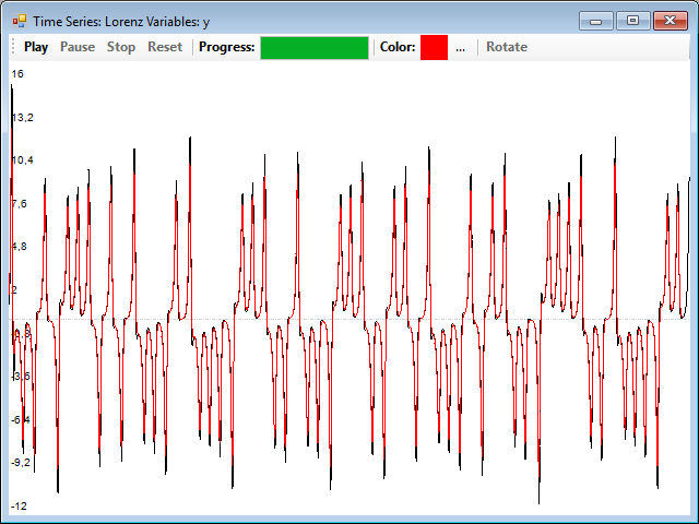
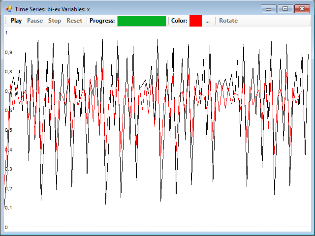
Really, the series of the variables X and Y in the Lorenz system are very similar, so this system is usually used as an example for this procedure. You can find another example in which the series no longer seem so much and also reconstructs the attractor quite well, with a distance of 1, if you load the bi-logistic.tsd file, and reconstruct the series from the Y variable. The reconstruction is quite good, but the series of the original X variable looks a bit more different that their reconstruction:
In the next and last article I will show you a sophisticated analysis tool, the recurrence plots.


