The back propagation algorithm
One of the most popular algorithms for training multilayer artificial neural networks is the back propagation algorithm, or retro-propagation algorithm. In this article I will try to explain its fundamentals, through a simplified implementation of a neural network that allows testing with different configurations of the network.
In this link you can download the source code of the BackPropagationDemo solution, with the code and data examples used in this article. It is written in csharp using Visual Studio 2017.
The code is based on the one in this post by Andrew Kirillov in CodeProject, although I have simplified it a lot to make it easier to focus on the learning algorithm.
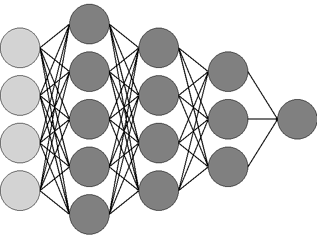
In order to apply this algorithm, the network must be a feedforward one, that is, it must have more than one layer of neurons and these must not form cycles; the outputs of one layer only feed the inputs of the next one, as in this figure:

The input data of the network is represented by the light circles on the left; the network has three hidden layers with 5, 4 and 3 neurons and an output layer with a single neuron. Each neuron has a single output, which is applied as input to all neurons in the next layer, and has as many inputs as the number of neurons in the previous layer.
Each neuron assigns a weight to each of its inputs, that is, it multiplies the value of each entry by a fixed amount depending on the importance assigned to it during the learning process; all these values, the entries multiplied by their weights, are added, and another value, called threshold, is added too to the result; this threshold is independent of the input and allows adjusting up or down the value of the sum of the entries times their weights. Each neuron implements an internal function that is applied to this sum to obtain the output result. Although each neuron can implement a different function, usually all of them use the same one; the function must be derivable in order to implement the backpropagation learning algorithm.
There are many appropriate functions to implement artificial neurons, I have chosen the bipolar sigmoid, whose result is bounded between -1 and 1 and has this form:
S(x) = (2 / (1 + e-αx)) – 1
Its derivative is as follows:
S’(x) = α (1 – x2) / 2
The α parameter allows us to configure the function by providing a scale factor that allows its slope to be more or less smooth.
The Neuron class
In the NeuralNetwork namespace, you will find the classes used to implement the neural network. The Neuron class implements the individual neurons, using the following data in its implementation:
private double[] _weights = null;
private double[] _weightUpdates = null;
private double _threshold = 0;
private double _thresholdUpdate = 0;
private double _alpha = 0;
private double _output = 0;
_weights is an array that contains the weights assigned to the inputs, while _threshold contains the threshold value of the neuron. _weightUpdates and _thresholdUpdate are used during the learning process to temporarily store the updates of the weights and the threshold. _alpha is the parameter to configure the sigmoid function, and _output is the value of the output, and is used to avoid performing redundant calculations.
When the neuron is created, the initial weights are randomly selected; the output value is calculated with the following methods:
public double CalculateOutput(double[] inputs)
{
    double sum = 0;
    for (int w = 0; w < _weights.Length; w++)
    {
        sum += inputs[w] * _weights[w];
    }
    _output = Sigmoid(sum + _threshold);
    return _output;
}
private double Sigmoid(double x)
{
    return (2 / (1 + Math.Exp(-_alpha * x))) - 1;
}
To the CalculateOutput method is passed an array with the values of the current inputs, and it returns the corresponding output value. The derivative of the function in the output, which will be used in the learning algorithm, is obtained from the Delta property:
public double Delta
{
    get
    {
        return _alpha * (1 - (_output * _output)) / 2;
    }
}
There are also some methods that will be used in the learning process to obtain and modify the weights assigned to the inputs:
public double GetWeight(int input)
{
    return _weights[input];
}
public double GetWeightUpdate(int input)
{
    return _weightUpdates[input];
}
public void SetWeightUpdate(int input, double update)
{
    _weightUpdates[input] = update;
}
public void ApplyUpdates()
{
    for (int w = 0; w < _weights.Length; w++)
    {
        _weights[w] += _weightUpdates[w];
    }
    Threshold += _thresholdUpdate;
}
The Layer class
Neurons are organized in layers. A layer is simply an array of Neuron objects, and it is implemented in the Layer class. The calculations required for the backpropagation algorithm are also implemented here. These are the data used in the implementation of this class:
private Neuron[] _neurons = null;
private Layer _prevLayer = null;
private Layer _nextLayer = null;
private double[] _outputs = null;
private double[] _errors = null;
private double _momentum = 0;
The _neurons array contains the neurons of the layer, and with _prevLayer and _nextLayer we have references to the previous layer and the next layer, which we will use in the process of learning and propagating the calculations when computing the inputs of the network to obtain the output. _outputs contains the outputs of the neurons in the layer, to avoid performing redundant calculations. The two remaining variables are used only during the learning process: _errors will contain the calculated errors for the output of each of the neurons in the layer, and _momentum is a parameter that allows us to configure the updating of the weights, as we will see when reviewing the algorithm itself.
There is a special constructor for the input layer and another one for the rest of layers. The difference is that the input layer does not have a previous layer, and the number of inputs per neuron is equal to the number of values that are presented to the network for each input vector, while the rest of the layers all have a previous layer and the number of entries per neuron is the number of outputs of that previous layer:
public Layer(int inputs, int neurons, double alpha)
{
    SetNeurons(inputs, neurons, alpha);
}
public Layer(int neurons, double alpha, Layer prevlayer)
{
    SetNeurons(prevlayer.OutputCount, neurons, alpha);
    _prevLayer = prevlayer;
    _prevLayer.NextLayer = this;
}
In order to process a data vector, the following method is used, which must be called only for the first layer, with the input data as a parameter:
public void Process(double [] inputs)
{
    for(int n = 0; n < _neurons.Length; n++)
    {
        _outputs[n] = _neurons[n].CalculateOutput(inputs);
    }
    if (_nextLayer != null)
    {
        _nextLayer.Process(Outputs);
    }
}
The results will be obtained by reading the outputs of the last layer.
The Network class
The Network class implements the whole neural network, as an array of Layer objects. This is the constructor, where everything is initialized:
public Network(int datainputs, int inputs, int outputs,
    int[] hidden, double alpha)
{
    _layers = new Layer[2 + ((hidden != null) ? hidden.Length : 0)];
    _layers[0] = new Layer(datainputs, inputs, alpha);
    Layer prev = _layers[0];
    if ((hidden != null) && (hidden.Length > 0))
    {
        for (int h = 0; h < hidden.Length; h++)
        {
            _layers[1 + h] = new Layer(hidden[h], alpha, prev);
            prev = _layers[1 + h];
        }
    }
    _layers[_layers.Length - 1] = new Layer(outputs, alpha, prev);
    _alpha = alpha;
}
The datainputs parameter contains the number of values that make up each input vector, inputs is the number of neurons in the input layer, outputs the number of neurons in the output layer, and the hidden array contains as many elements as hidden layers are, each one with the number of neurons corresponding to the layer; this parameter can be null, in which case the network will only have an input layer and an output layer. The alpha parameter is used to initialize the neurons.
To process an input vector, or an array of vectors, the following methods are used:
public double[] Compute(double[] inputs)
{
    _layers[0].Process(inputs);
    return _layers[_layers.Length - 1].Outputs;
}
public double[][] Compute(double[][] inputs)
{
    double[][] result = new double[inputs.Length][];
    for (int ix = 0; ix < inputs.Length; ix++)
    {
        _layers[0].Process(inputs[ix]);
        result[ix] = new double[_layers[_layers.Length - 1].Outputs.Length];
        _layers[_layers.Length - 1].Outputs.CopyTo(result[ix], 0);
    }
    return result;
}
Which receive as a parameter the network inputs and return the corresponding outputs.
The backpropagation algorithm
Let's finally go to the algorithm itself. I will try to explain it without using mathematical formulations, from which you can find a lot by searching on internet, since I try to convey a practical understanding of the procedure.
To train the network, we take a set of data with a number m of samples. Each sample consists of some values corresponding to the inputs and values that correspond to the outputs we expect to obtain; the backpropagation algorithm is of the type of learning we call supervised, since we need to know in advance the output we want to obtain. The algorithm proceeds in the following way for each of the samples:
- Calculate the output value of the network from the input values.
- Starting from the output layer, calculate the error committed between the actual output and the one provided by the network.
- This error propagates back to the previous layer, which also calculates an error value for each neuron from the errors of the next layer. In this step we obtain the current error of the network, from which we obtain the average for all the samples.
- Once the errors for all the layers have been calculated, the necessary updates for the weights of the neurons of each layer are calculated. In this phase there are two configurable parameters: the learning rate, which allows making these updates in more or less small steps, and the momentum, which allows taking into account the value of the previous weight update. By playing with these two values, we can fine-tune the learning process.
- Finally, these updates are applied to all neurons in the network.
Once all the samples have been processed, if the average error is lower than a prefixed value, or if we have already processed the whole data set a maximum number of times, the algorithm ends and the network is trained.
In the code, this is the method of the Network class that processes each sample:
private Task<double> TrainSample(double[] inputs,
    double[] finaloutputs, double learningrate)
{
    return Task.Run(() =>
    {
        _layers[0].Process(inputs);
        double error = _layers[_layers.Length - 1].ComputeError(finaloutputs);
        _layers[0].ComputeUpdates(inputs, learningrate);
        _layers[0].ApplyUpdates();
        return error;
    });
}
As parameters, it receives the input values in the inputs parameter, the expected output values in finaloutputs and the learning rate in learningrate, this rate is usually less than 1, in the order of 0.001 or 0.01. The network error for the current sample is calculated starting with the output layer, calling the ComputeError method of the Layer class:
public double ComputeError(double[] finaloutput)
{
    double error = 0;
    for (int n = 0; n < _neurons.Length; n++)
    {
        double e = finaloutput[n] - _outputs[n];
        _errors[n] = e * _neurons[n].Delta;
        error += e * e;
    }
    _prevLayer.ComputeError();
    return error / 2;
}
For each neuron in the layer, the difference between its current output and the expected output is calculated; the error in the output layer for this neuron is the product of this difference and the value of the derivative of the neuron's function at the point of its current output. This value is stored in the _errors array as the error corresponding to the current neuron. The error variable, on the other hand, will contain the mean square error of all the neurons of the output layer, which is the value that we will consider as network error for the current sample.
From the last layer we will calculate the error of the previous layer, with another version of the ComputeError method, since in the rest of the layers the calculation of the error is done in a different way:
private void ComputeError()
{
    for (int n = 0; n <_neurons.Length; n++)
    {
        double esum = 0;
        for (int e = 0; e < _nextLayer.Errors.Length; e++)
        {
            esum += _nextLayer.Errors[e] * _nextLayer.GetWeight(e, n);
        }
        _errors[n] = esum * _neurons[n].Delta;
    }
    if (_prevLayer != null)
    {
        _prevLayer.ComputeError();
    }
}
In the rest of layers, we don't know what the correct final value should be, so what we calculate is the sum of the product of the error of each neuron in the next layer by the weight that this neuron has assigned to the output of the neuron whose error we are processing. Again, we multiply this error by the derivative of the neuron function at the point corresponding to the current output to calculate the final error of the neuron in the current layer. From here, the procedure is the same to calculate the errors of the rest of the layers, until arriving at the first, where the process stops.
With all the calculated errors, the next step is to calculate the value of the update for each one of the weights. This process begins in the first layer, the input layer, passing the current sample data in the inputs parameter of the ComputeUpdates method of the Layer class:
public void ComputeUpdates(double[] inputs, double learningrate)
{
    for(int n = 0; n < _neurons.Length; n++)
    {
        for (int w = 0; w < _neurons[n].InputCount; w++)
        {
            _neurons[n].SetWeightUpdate(w, learningrate *
                (_momentum * _neurons[n].GetWeightUpdate(w) +
                (1 - _momentum) * _errors[n] * inputs[w]));
        }
        _neurons[n].ThresholdUpdate = learningrate *
            (_momentum * _neurons[n].ThresholdUpdate +
            (1 - _momentum) * _errors[n]);
    }
    if (_nextLayer != null)
    {
        _nextLayer.ComputeUpdates(Outputs, learningrate);
    }
}
We process each neuron in the layer, and for each neuron, the weight of each input. The parameter _momentum can take any value between 0 and 1, so that we distribute the updating amount between two factors: on the one hand, the value of the last update that we have calculated for this weight ((_momentum * _neurons [n] .GetWeightUpdate (w)) and, on the other hand, the error of the neuron multiplied by the value of the corresponding input ((1 - _momentum) * _error [n] * inputs[w]). The value of _momentum determines whether we take into account, and to what extent, the past updates
With the learningrate parameter we make this update more or less slow, to finely adjust the accuracy and speed of learning. The calculation continues on the next layer, this time with the outputs of the current layer as input values.
Finally, the changes are applied to all the neurons, also starting from the first layer, with the ApplyUpdates function:
public void ApplyUpdates()
{
    for(int n = 0; n < _neurons.Length; n++)
    {
        _neurons[n].ApplyUpdates();
    }
    if (_nextLayer != null)
    {
        _nextLayer.ApplyUpdates();
    }
}
The BackPropagationDemo application
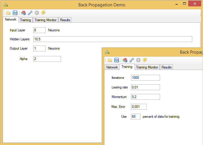
As a demonstration of the use of this algorithm, I have prepared the BackPropagationDemo application, with the following user interface:

In the toolbar, from left to right, there are the following command buttons:
- Open file: allows loading data in csv format or neural networks already trained by the program.
- Save: Allows the current network to be saved in a binary file.
- Build Network: Builds a new appropriate network for current data.
- Train: Train the network with the current parameters and current data.
- Stop Training: stop the learning process before it ends.
- Process Data: it allows processing the loaded data from a file and shows the results.
The first tab, Network, allows you to enter the parameters of the network. Always indicate an input layer and an output layer, each one with the number of neurons in them, but bearing in mind that we will reserve as many values at the end of each row of data loaded as neurons we have selected for the output layer. The rest of the values will be used as inputs. If we want to add hidden layers, we can do it by providing a comma separated list of values.
Training parameters are provided on the Training tab. The maximum number of iterations, indicates how many times the network has to process the complete set of data used for training; the parameters learningrate and momentum have the meaning indicated above; Maximum error provides a minimum acceptable error level to stop the training process before finishing all iterations. Finally, we indicate, for the data set that we are going to load in a csv file, the percentage of samples that will be used for the training. This value must be indicated before loading the data.
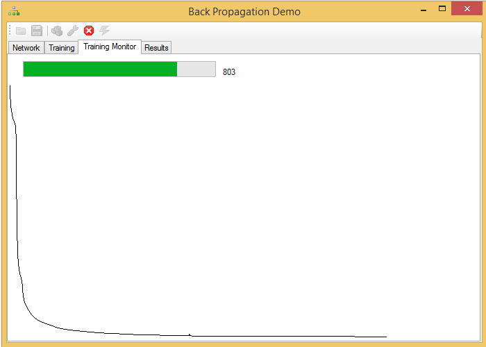
While training the network, we can continue interacting with the program, seeing a graph with the variation of the network error and the iterations made:

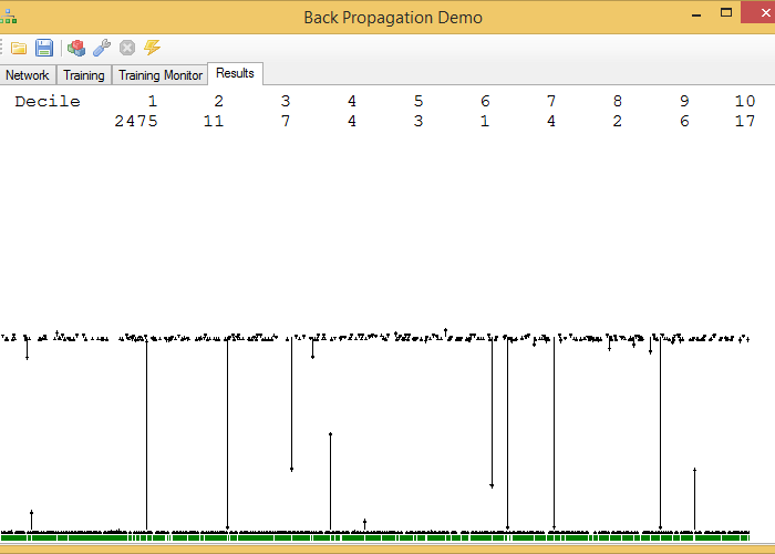
Finally, once the network is trained, we can check the result by processing the data that has not been used for the training:

This graphic is not a very orthodox one. In the upper part are the quantities of samples whose expected value has a difference with the value provided of the network lower than n / 10 parts of the maximum error committed by the network. In the capture, for example, there are 2474 samples with an error less than 1/10 of the maximum error.
The graph of the lower part represents the differences for each sample between the actual and calculated values, with an arrow that starts from the actual value and ends, as an arrow, in the value calculated by the network. These graphs only make sense for networks with a single output neuron.
I have added two sets of data that can be used to perform tests, iris.csv, obtained from the R application, with 4 data values and a result value for three lily species, and postures.csv, with 20 data values and one of result, which represent values of two different positions obtained with the Microsoft Kinect sensor, according to the normalization of the posture that I provided in these articles.
All the data loaded in the program is scaled within the interval (-1, 1), regardless of its value.


