WinRQA, a C# application to draw recurrence plots

A recurrence plot is a graphical tool used in the study of complex time series. Along with the plot we can also calculate a series of measures that allow us to perform a recurrence quantification analysis, or RQA. In this article I will present the WinRQA application, a tool to work with recurrence plots and RQA measures in a Windows environment.

In this blog I have already treated in other articles on this subject, in this link you can see an introduction to recurrence plots. I can also recommend this website entirely devoted to recurrent plots, or this book about recurrence quantification analysis.

In this link you can download the executables of the WinRQA application, and, in this another one, you can download the source code of the WinRQA project, written in csharp with Visual Studio 2013.

The application works in any version of Windows from Windows 7, possibly also in Windows Vista, although I have not been able to test it in this version.

The WinRQA application

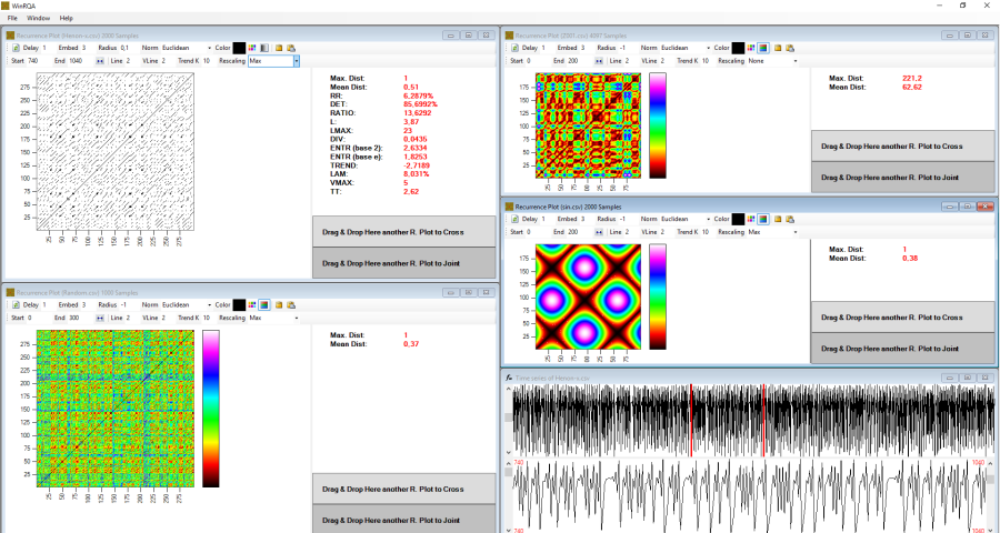
WinRQA is an MDI application, so you can work with multiple recurrence maps at the same time. At the moment it only works with text files. These files must contain a value of the time series in study per line, and should not have any line or column header.

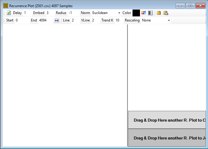
To load a data file, simply select the Open option from the File menu. A window will open where you can parameterize the recurrence plot for their visualization:

There are two toolbars with which we can parameterize the recurrence plot. From top to bottom and from left to right we can find the following parameters:

• Delay: here we indicate the displacement that we want to apply to extend the dimension of the series. Recall that each extra dimension we want to add to the time series is constructed taking the values of the original series starting with the element that is displaced n delays from the initial position, where n is the index of the new dimension. It must be an integer greater than or equal to 1. Its maximum value is limited by the size of the series and the embedding dimension.
• Embed: here we indicate the embedded dimension that we guess the series has, that is, the number of dimensions to which we want to extend it. The minimum value is 1, meaning that we study the time series without adding new dimensions. The maximum value is limited by the size of the series and the selected delay.
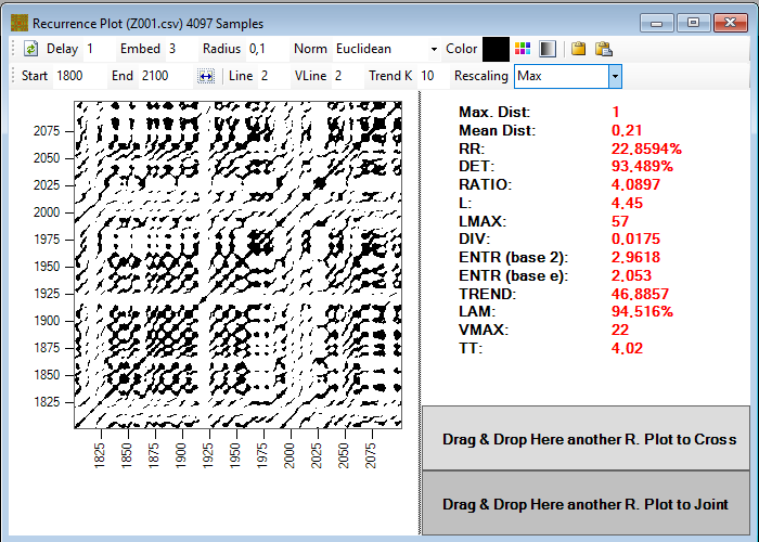
• Radius: The recurrence plot is built based on the distance between the different points in the series. We can represent these distances in the form of a gradient, using a color or gray scale to indicate the relative distance between each pair of points, or indicate a threshold below which two points are considered recurrent (they are located in the same place as the phase space), and above which it is considered that the points are not recurrent. In the latter case, what we represent is a bicolor map in which points of recurrence are highlighted. If we provide a radius less than zero, the plot will be drawn with a color gradient, whereas if we provide a value greater than or equal to zero, we will get a two-color recurrence plot. RQA measurements will only be calculated for maps with a radius greater than or equal to zero.
• Norm: Since what we do to construct the map of recurrence is to calculate the distances between the different points of the same, we must define how we are going to calculate this distance. There are three possibilities, we can use the Euclidean distance, or to use the maximum or the minimum distance between the coordinates of each pair of points.
• Start and End: With these parameters we define the window inside the series that we are going to use to draw the recurrence plot; they simply indicate the index of the initial and final elements of the series corresponding to the first dimension. It must be taken into account that at the end of the series must remain (E - 1) * D elements, being E the embedded dimension and D the delay, in order to construct the extended series.
• Line: This is a parameter for calculating RQA measures. It defines the minimum length that must have a diagonal line of recurring points to be taken into account. Usually the minimum value, which is 2, is used.
• VLine: same as above, but referring to vertical lines.
• Trend K: To calculate the TREND measure a constant must be defined to indicate the number of lines that are taken into account from the main diagonal (LOi or Line Of identity).
• Rescaling: since the application allows performing joint or crossing recurrence plots between two series, we can use the rescaling option to normalize the distance values so that they are comparable. Along with the option of not rescaling, we can divide all distances by the maximum one, to get values between 0 and 1, or by the average distance, to smooth the range of values.

There are also a number of command buttons. Again from top to bottom and from left to right, we have the button to draw the map and recalculate the RQA measures with the provided parameters. In the case that we are visualizing a cross or joint plot, the normal recurrence plot of the series with itself will be redrawn.

With the button you can select the color with which recurrent points will be represented when drawing a two-color map, while the button allows us to select a gray or color scale to represent the plot in the form of a gradient of distances.

The button will copy the recurrence plot image to the clipboard, while the button will copy a table with the RQA measures, using tab characters as column separators. In this way we can export the results to other programs.

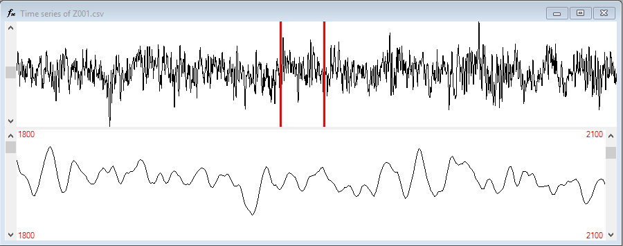
Finally, the button allows you to display the time series to select the start and end of the window to draw the plot. The following window will be shown:

At the top of the window is the complete series. We can select the start point with the left mouse button and the end point with the right one. The scroll bar on the left can be used to move the window through the series without varying its size.

At the bottom is the part of the series that we have selected, the side scroll bars can be used to fine-tune the start and end positions of the window.

The changes we make in this window are immediately reflected to the Start and End text boxes, although to see the resulting plot you must use the button.

Finally, we can drag a plot and drop it on another to display a cross-recurrence or a joint-recurrence plot. To do this, there are two panels on the right side of the plot window. The plots for cross-recurrence must have the same dimension. In addition, the map that we drop must have a window size equal to or greater than that of the plot with which we want to cross it.

With the joint plots, the dimension constraint does not apply.

In this other link you can find the source code of WinRQA commented in CodeProject.

To end, in this link you can find the first extension of the WInRQA application features, with tools to help estimate the correct delay and embedding dimension for the recurrence plot.