Tableaux for first order logic

The Tableaux is a logical calculation tool that allows checking the validity of a conclusion from a series of premises. In the previous article I explained briefly the fundamentals of Tableaux for predicate logic. In this article I will extend the program to the first-order logic, which has much more expressive capacity than predicate logic, although this makes also automatic calculation more difficult.

In this link you can download the project FOTableaux with the source code and the executable program written in CSharp with Visual Studio 2013.

Let's start with a review of the elements of first-order logic. First, we have the terms:

Constants, which represent a particular individual and that, in the program, must be written always starting with the character '_', followed by a letter and any number of alphanumeric characters. They can also be used as constants the natural numbers.
Variables, representing a generic individual. The program differentiates the variables of the constants because his name does not begin with the character '_', but by a letter followed by any number of alphanumeric characters.
Functions, which are compound terms, as they have parameters that must be also terms. In the program, the functions are written with a name that begins with any letter followed by any number of alphanumeric characters and a list of parameters separated by commas enclosed in parentheses, for example: f(x, y, _c). The result of a function is an individual, that is, a term. For example "the father of x" is a function.

The formulas are constructed using the following elements:

The symbols True and False are formulas.
A proposition or relationship relative to 0 or more terms is a formula. They should be written with a letter followed by any number of alphanumeric characters, with the list of terms to which it references separated by commas enclosed in brackets. The brackets should be placed although the proposal has no parameters. For example, "x and y are friends" is a relationship, and should be written FR[x, y].
An equality is a formula. It consists of two terms connected with the = operator, for example x = y.
A formula to which is applied the NOT logical negation operator, is a formula.
Two formulas connected by the logical operators AND, OR, implication and double implication is also a formula.
There are some elements, called quantifiers, which refer to a particular variable in a formula and can refer to all possible individuals (universal quantifier) or only to one or more individuals (existential quantifier). A formula on which they apply a quantizer is also a formula.

Although the use of the program in this version is basically the same as in the previous article, I modified the symbols that appear in formulas so that they are written in a standard format; these are the keyboard keys and the symbols that they give:

AND operator, is obtained by pressing the & key, but the symbol that appears is the ˄ character.
OR operator, is obtained by pressing |, but the symbol that appears is the character ˅.
Implication: pressing the < key the character → is obtained.
Double implication: pressing the > key the ↔ character is obtained.
Universal quantifier: it is obtained by pressing the @ key.
Existential quantifier: it is obtained by pressing the # key.
True, it is obtained by pressing the $ key, the symbol is ⟙.
False, it is obtained by pressing the % key, the symbol is ⟘.

Parentheses can be used to group formulas. For example, is not the same PT[x] → (PQ[x]˅PL[x]˅SV[x]) than PT[x] → PQ[x]˅PL[x]˅SV[x] as, in this program, the implication operator has higher precedence than the OR or AND operator.

Equalities must be enclosed in parentheses if you want to negate them. In general, it is best to always write the equalities in parentheses.

Parentheses are also used to apply a quantifier to a composite formula, such as ᗄx(PT[x] → (PQ[x]˅PL[x]˅SV[x])). If you do not put parentheses, the quantizer only applies to the first sub-formula, PT[x].

The program always transforms the implications in their equivalent formulas using the AND and OR connectives and the NOT operator. It also solves the negations of composite formulas before processing the Tableaux.

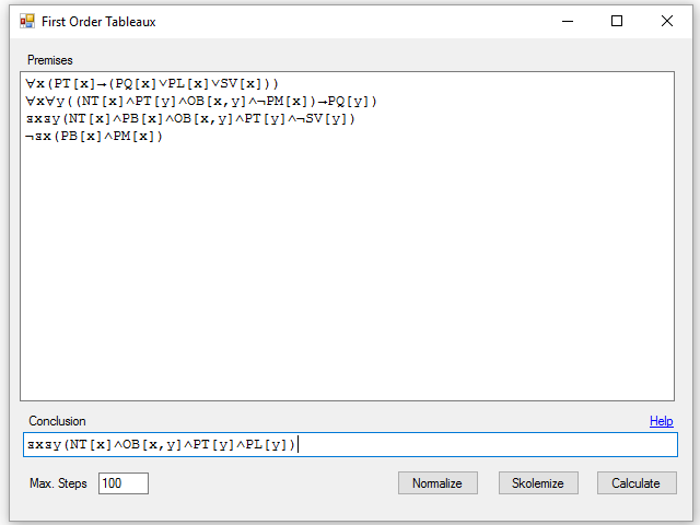
This is the program look:

To the functionality of the Tableaux for predicate logic I have added the following:

Maximum number of steps (Max Steps). A first order Tableaux can be infinite. It is also possible that, with a very complex set of formulas, the program will not be able to find the proper development to end the Tableaux. To prevent the program from hanging up, you can specify the maximum number of formulas to create until the program ends.
Normalize. With this button, all formulas are rewritten in prenex normal form, which involves passing all quantifiers to the beginning of the formula. There is no need to use this option to calculate the Tableaux, but you can use it to correct exercises, for example.
Skolemize: it involves passing formulas to Skolem normal form that is a prenex form where existential quantifiers have been eliminated and their quantified variables are replaced by constants or appropriate functions. The constants and functions introduced in this step are named using the following structure: *sk + order number. To calculate the Tableaux is not recommended to use the standardized Skolem formulas, since the substitution of variables and functions is performed at each formula independently of the others, and it can change the meaning of the argumentation. This option can be used to correct exercises, by example.

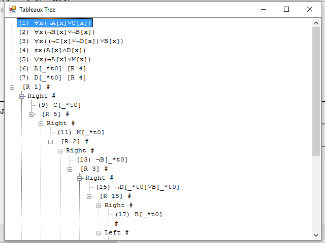
As a result we obtain the Tableaux displayed in two different formats, more or less appropriate depending on the size of the result. On one side, a tree view is shown, in which the branches can be expanded or collapsed and that contain the formula list in the nodes of the Tableaux branches, this view is more appropriate for large sets of formulas.

The closed branches are indicated by the # symbol, as in the Tableaux for predicate logic, and the number of the formula that has been used to create new ones or make a branch is indicated in brackets after the letter R.

The existence of the equality operator introduces two new rules for creating formulas. On the one hand there is the rule of reflexivity, indicated by the letters RF which allows you to enter at the end of a branch the formula t = t, where t is a term any of those in the branch. We can also use the substitution rule, indicated by the letters ST, which allows us to replace in a formula of the branch the term t by the term t', provided there is a formula of the form t = t' in the branch.

To create new formulas from formulas with quantifiers, in the case of existential quantifiers, we replace the variable quantified by a new constant, called example, which has not been already used in the branch. There can't be more than one example of existentially quantified formula in the same branch. Quantified variables by the universal quantifiers can be substituted by any term present in the branch or by a new constant, if there is no term available. These constants, or functions, introduced to particularize quantified formulas are always named following the scheme *t + sequential number.

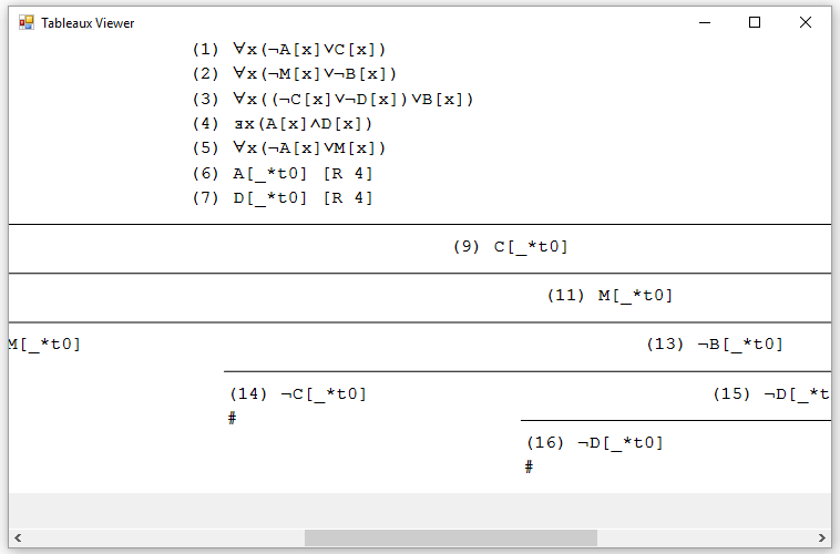
We also get a view of the Tableaux fully expanded that can be useful when the number of formulas is not too high:

This Tableaux can also be used to solve any problem of predicate logic, since it is a subset of first-order logic. However, the heuristics used to try to resolve the first order Tableaux doesn't goes beyond the next step, so that the algorithms may have to be quite improved for solving problems with complex sets of formulas. The program successfully solves all the exercises in the book that I used as a reference, and which is as follows (sorry, only in Spanish): Mathematical logic for informatics.