Recurrent neural networks and time series
The recurrent neural networks are a very appropriate tool for modeling time series. This is a type of network architecture that implements some kind of memory and, therefore, a sense of time. This is achieved by implementing some neurons receiving as input the output of one of the hidden layers, and injecting their output again in that layer. In this article I will show a simple way to use two neural networks of this kind, the Elman and Jordan ones, using the R program.
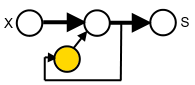
In the Elman networks, the inputs of these neurons are taken from the outputs of the neurons in one of the hidden layers, and their outputs are connected back to the inputs of the same layer, providing a memory of the previous state of this layer. The scheme is as in the figure below, where X is the input, S the output and the yellow node is the neuron in the context layer:
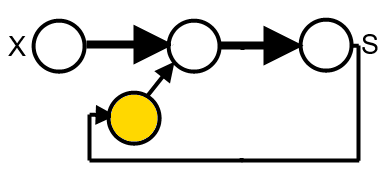
In the Jordan networks, the difference is that the input of the neurons in the context layer is taken from the output of the network:
Precisely for this memory feature, they are suitable for modeling time series. Let's see how to use it with the R program. First, you must load the packages that implement these neural networks. I will use the package RSNNS and, secondarily, the quantmod package for some operations.
As an example of time series, I will use first a series generated by the logistic function in the domain of chaotic dynamics. The chaotic dynamics gives the series a complex structure, making the prediction of future values very difficult or impossible. This series is obtained using the following equation:
Xn+1 = µXn(1-Xn)
When the μ parameter takes values approximately over 3.5, the dynamics of the series generated becomes chaotic. In this link you can download a csv file with 1000 values of the logistic series, using an initial value of 0.1 for X and a value of 3.95 for μ.
You have to start loading the packages and the series data:
require(RSNNS)
require(quantmod)
slog<-as.ts(read.csv("logistic-x.csv",F))
The values of the logistic equation are all in the range (0,1) and this does unnecessary to preprocess them, otherwise, it is convenient to scale them. As we have 1000 values, we will use 900 to train the neural network. To do this we define the train variable:
train<-1:900
Let's define as series training variables, the n previous values of it. The choice of n is arbitrary, I selected 10 values, but, depending on the nature of the problem we are dealing with, can be convenient another value. For example, if we have monthly values of a variable, 12 might be a better value for n. What we'll do is create a data frame with n columns, each of which is constructed advancing a value of the series in the future, through a variable of type zoo:
y<-as.zoo(slog)
x1<-Lag(y,k=1)
x2<-Lag(y,k=2)
x3<-Lag(y,k=3)
x4<-Lag(y,k=4)
x5<-Lag(y,k=5)
x6<-Lag(y,k=6)
x7<-Lag(y,k=7)
x8<-Lag(y,k=8)
x9<-Lag(y,k=9)
x10<-Lag(y,k=10)
slog<-cbind(y,x1,x2,x3,x4,x5,x6,x7,x8,x9,x10)
We eliminate the NA values produced by shifting the series:
slog<-slog[-(1:10),]
And we define, for convenience, the input and output values of the neural network:
inputs<-slog[,2:11]
outputs<-slog[,1]
Now we can create an Elman network and train it:
fit<-elman(inputs[train],
    outputs[train],
    size=c(3,2),
    learnFuncParams=c(0.1),
    maxit=5000)
The third parameter indicates that we want to create two hidden layers, one with three neurons and another one with two; I have indicated a rate of learning of 0.1, and also a maximum number of iterations of 5000. With the function plotIterativeError can see how it has evolved the network error along the training iterations:
plotIterativeError(fit)
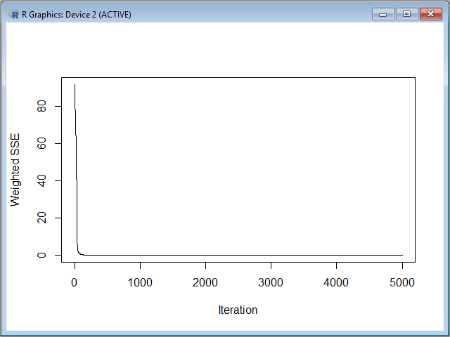
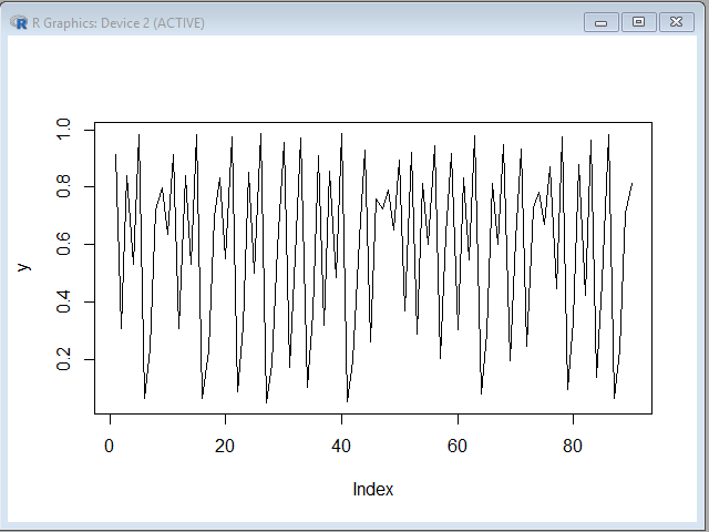
As we can see, the error converges to zero very quickly. Now let's make a prediction with the remaining terms of the series, which has the following graphical appearance:
y<-as.vector(outputs[-train])
plot(y,type="l")
pred<-predict(fit,inputs[-train])
If we superimpose the prediction over the original series, we can see that the approximation is very good:
lines(pred,col="red")
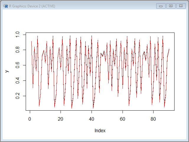
At this point, the question that may arise is: have we made a perfect prediction of a chaotic series? but is not that impossible? The answer is that what really happened here is that the neural network has "learned" the logistic function perfectly, and is able to predict fairly well the next value of any other.
In fact, all predicted values have been made from 10 previous actual values of the series, if you try to predict new terms using as input values other previously predicted ones, due to the chaotic nature of the series and their sensitivity to initial conditions, the accuracy is quickly lost, which is consistent with the chaos theory in that chaotic phenomena are only predictable in a very short time. In any case, thanks to the memory effect, we can anticipate the series in at least one value with very good accuracy, which can be very useful in some applications.
If we want to perform the same test with a Jordan network, the command to use is as follows:
fit<-jordan(inputs[train],
    outputs[train],
    size=4,
    learnFuncParams=c(0.01),
    maxit=5000)
With this command we have requested four hidden layers and a learning rate factor of 0.01. The result is also adjusted quite well to the original series:
pred<-predict(fit,inputs[-train])
plot(y,type="l")
lines(pred,col="red")
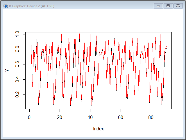
As the series generated by the logistic equation, in the chaotic domain, is sensitive to initial conditions, you can generate another series with the same parameter but starting with a different value instead of 0.1, within the range (0,1). This will generate a totally different series that the one we used to train the network, and you can see that the model is able to predict also the values of the section of the new series we want, which indicates that the model has "learned" well the logistic equation that generates the series.
The logistic function generates a series of a single variable. Let's test the network with a system of two equations with two variables, the Henon system, which also generates time series with chaotic dynamics, with these equations:
Xn+1=1+Yn-1.4Xn2
Yn+1=0.3Xn
In this link you can download the series with 1000 terms of the x variable of the Henon system in csv format. Now we have a series that depends on two variables, generated by a system of which we have incomplete information because we only have the series of one of the two variables. We can repeat the above procedure:
shen<-as.ts(read.csv("henon-x.csv",F))
y<-as.zoo(shen)
…
inputs<-(inputs - min(y))/(max(y)-min(y))
outputs<-(outputs - min(y))/(max(y)-min(y))
In this case, the series values are between -1 and 1, so that we have to standardize to in order to take values between 0 and 1, as, doing this, the model fits best.
And, again, we perform a prediction of the remaining series values:
pred<-predict(fit,inputs[-train])
y<-as.vector(outputs[-train])
plot(y,type="l")
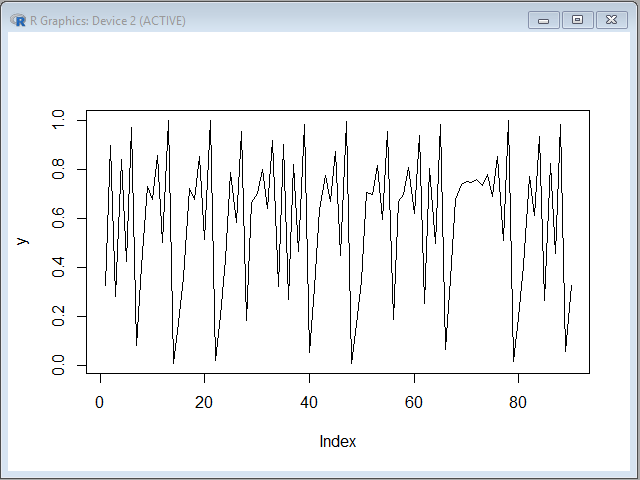
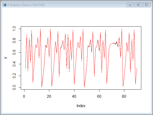
We can check that the fit is almost perfect:
lines(pred,col="red")
Finally, I am going to recommend a book about working with neural networks with the R program: Deep learning made easy with R, of N.A. Lewis, which explains in a simple and convenient way the main types of neural networks and their applications.


