Time series, RQA and neural networks I

In some other articles in this blog, I have already written about complex time series, recurrence quantification analysis (RQA) and neural networks. In this series of articles, I will discuss some points to take into account when combining the use of these two tools to identify patterns in complex series, such as detecting anomalies in electrocardiograms or electroencephalograms.

If you google the terms RQA and DNN, you will find many articles and papers about studies that combine both tools. With the recurrence quantization analysis, we can codify any time series of any length into a set of around 10 numbers that quantify different properties of that series. With neural networks, we can use this set of values to find patterns in order to identify different cases, such as abnormal functioning of the organism, differentiating one person from another, or determining if the subject in study is performing certain activity, among a given group of them.

Recurrence Quantification Analysis (RQA)

The idea underlying RQA is as follows: first, we conjecture that a complex time series only shows a part of a certain system. For example, if we have a population of wolves in a given territory and we take data on the variation of the population over time, we will obtain a time series, but the wolves are predators, and they obtain their food by hunting other animals, such as rabbits. The variations in the population of wolves will surely be tightly correlated with variations in the population of their prey, and, in turn, if their prey are herbivores, for instance, their population will be correlated too with that of edible plants. If instead of having only the population series of the wolves we also had the populations of the rabbits and the carrots, we could understand much better the dynamics of the whole system.

These populations are not only related, but they influence each other, with a certain delay in time: if the number of rabbits increases, shortly thereafter increases the number of wolves, and the availability of carrots will reduce. We can think on each of these series as dimensions of the whole system. In this case, the system would have three dimensions, but we can have systems with any number of them. Some results of the algebraic topology, such as Whitney theorem, allow us to affirm that we can reconstruct the complete system in an approximate way, conserving its principal properties largely, although we only have one of the series or dimensions that compose it. The procedure is simple: we calculate a certain delay of time t, which will depend on our system in question, and replace the n - 1 dimensions that we assume are missing by a copy of the series of the previous dimension, but starting at the element in the t position. Suppose we consider that the delay t is 30 days, the population of wolves will be the series that we already have, without changes. For the population of rabbits we will take the series of the wolves, but starting with the element corresponding to 30 days from the beginning of the series, and for the carrots population, we will start 60 days after the start.

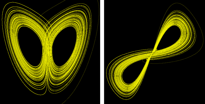
With this procedure, the elements of the series now have three components: one that represents the wolves, another the rabbits and another the carrots. Speaking in abstract terms we can say that the series that characterizes the system consists of points with three coordinates x, y, z. If now we represent this series as a trajectory in a three-dimensional space, we would obtain what is known as the attractor of the system. As we do not have this series of populations of wolves that we are using as an example, we can get an idea of that by reconstructing the Lorenz attractor, which is the attractor of a three-dimensional system whose series can be easily obtained. We will reconstruct it using only the series corresponding to the x component:

On the left side is the original attractor, and on the right side, the reconstructed one. It is not perfect, but its topology is similar to the original.

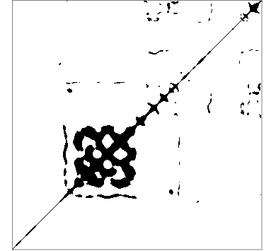
The recurrence quantification analysis can begin from a series of just one dimension and extends it to more dimensions. The final number of dimensions is a parameter known as the embedded dimension. The delay used to build the additional dimensions is another of the main parameters. The aim of this tool is to find the points of the attractor by which the portion of the series under study passes more than once or, more strictly, passes through its vicinity. The third parameter that we must provide for this analysis is, therefore, the maximum distance that separates two points considered recurrent, which is also known as radius. Once decided the values of these parameters, a rectangular matrix is constructed in which the rows and columns correspond to the different points of the series, ordered in time. Using the index i for the rows and j for the columns, the element i, j of the matrix is set to 1 if the distance between point i and point j of the series is less than the radius (recurrence point), or 0 otherwise. If we draw this matrix using black for the recurrence points and white for the rest, we will obtain a recurrence plot, which may look similar to this one:

The points on the diagonal are always recurrent, because they represent the recurrence of a point with itself. From this plot, we can calculate measures such as the proportion of recurrence points over the total points (RR); the proportion of recurrent points that form continuous diagonal lines (DET); the proportion that forms vertical lines (LAM); the average length of the diagonal lines (L); the average length of the vertical lines (TT); the maximum length of the diagonal and vertical lines (LMAX, VMAX); the inverse of LMAX (DIV) and other measurements slightly more complicated to calculate (RATIO, ENTR, TREND). You can find a much better and rigorous approach on this subject in this website entirely devoted to recurrent plots.

The fact is that, this way, we have a criterion to characterize any section of a time series, and therefore its dynamics, using this series of measurements, which can also be used to detect important changes in this dynamics.

This is equivalent to identifying and classifying patterns, and, for this task, we have a tool widely documented and implemented in many environments, with code libraries available for many languages. They are relatively easy to implement by oneself, as well: neural networks.

However, you have to be careful when using these two tools combined, because things are not as easy as they might seem at first. It is easy to get results that seem conclusive at first sight, but that can lead us to absolutely wrong conclusions or to believe that we are seeing things in the data that really are not there.

In order to illustrate this issue, I will use the R environment to work with time series taken from a dynamic system with a turbulent regime and, therefore, with a certain degree of caoticity, such as the human heart. Specifically, we will use electrocardiograms (ECG), from the PhysioNet database. All the code and data files needed to reproduce the examples of this series of articles can be downloaded using this link. Although I provide the data already processed, you can find the original files in PhysioNet, in this link. In this article about working with files in EDF format, you can find information on how to download and process the original data from PhysioNet.

You have to load the following libraries in the R environment, in order to execute the examples:

library(edfReader)
library(crqa)
library(RSNNS)

The first one allows to read EDF files, the second one calculates RQA measurements, and the third one allows implementing neural networks.

Electrocardiograms (ECG)

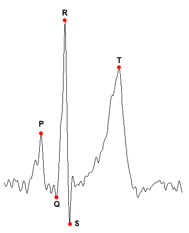
An ECG is a continuous signal that represents the electrical activity of the heart over time. Each beating looks similar to this:

The points P and T represent the maxima of the so-called P and T waves, while the points Q, R and S form the so-called QRS complex, which corresponds to the contraction of the ventricles. These points and their relationships are used in the usual interpretation of an ECG. In this case, we are only going to be interested in point R, since we are going to transform the complete wave in its corresponding RQA measurements and this point is the easiest to detect. It will be used to select sections of the ECG representing complete beats.

When working with physiological signals in general, we must take into account some issues:

• Sampling rate: if we compare two ECGs, we must ensure that the time scale of both is the same.
• The different derivations of the ECG: the ECG is obtained from several electrodes located in different positions of the chest, arms and legs. A derivation is the voltage difference voltage between two electrodes, so there may be different derivations, or signals, in the same record, which can be quite different among them, although the beats are in all of them in the same position. Comparing different derivations of two ECGs may not be a good idea.
• The voltage of the signal: not all ECG have the same voltage levels. It may be necessary to scale the signals to standardize voltage ranges.
• Noise: some ECGs present different levels of noise component; sometimes the signal has undulations instead of having a straight basal line. Recurrence analysis is quite sensitive to noise, which can completely distort the results.
• Inversion of signals: some ECG registers record the signal with inverted polarity, so you have to make sure to invert it again to compare it with the other signals.

Having all this in mind, in the next article we will start working with the signals.