Time series, RQA and neural networks II

In this second article in the series on combining recurrence quantification analysis (RQA) and neural networks to work with complex time series, we will examine some ideas about possible processing that you can apply to the data and the selection of parameters. We will work using electrocardiographic signals, as mentioned in the previous article.

In this link, you can access the first article in this series, where you can find a general introduction on the subject. You can download the examples of code and data that I will use by using this link.

The electrocardiograms that we will use are from the PhysioNet database of physiological signals. It includes several pairs of electrocardiograms from a number of subjects. There is an electrocardiogram for each subject corresponding to a normal state, without any special activity, and another one taken during the performance of different arithmetic calculation tasks. All the subjects are healthy, and you can find some information about them in the file subject-info.xlsx.

The name of the subjects data files is composed with the word Subject followed by a two-digit number. The normal electrocardiogram identifier is the number 1, and the number 2 identifies the file corresponding to the ECG obtained during the arithmetic tasks. We also have the age, the gender and the number of calculations performed correctly for each subject, which provides a measure of the difficulty of the task for that individual. All time series were been recorded using the same sampling frequency, so no modification is necessary at all.

The original data format is the EDF format, but I have recorded the ECGs I will use as csv files to simplify its handling. I have selected only women and only the electrocardiograms that correspond to calculation tasks. The objective is to compare a group that has obtained good results with another group that has obtained bad results, and see if we can differentiate them based on the results. We will also try to apply the networks trained in this way to identify complete electrocardiograms not used in the learning process.

Since these are healthy subjects, the only reasonable assumption in order to differentiating one group from the other seems to be that the heart rate may be different. Recurrence analysis provides us with information about the dynamics of a series, and the dynamics of the heart does not change when we are making simple calculations. What would be expected from this analysis is that the results do not show differences between both groups, but the thing is not so simple. Neural networks are very effective in finding differences in a set of data separable into classes, even arbitrarily, especially if those classes are linearly separable. On the other hand, RQA is quite sensitive to small inevitable differences between heartbeats, even simply to noise, so spurious differences appear very easily, and can complicate things a lot.

Preparing the data

Let us start by loading the libraries and the necessary code for the examples:

library(crqa)
library(RSNNS)
source(“ecgtools.r”)

The last file can be found among the code examples and has some useful functions to work with signals. When transforming a time series into a set of RQA measurements, one of the things to decide is the data window to be used, the length and starting position of the portion or portions of the series. The longer these portions are, the longer it will take to perform the analysis, and the results will be different with different portions and different lengths. In an electrocardiogram, it seems natural to use the heartbeat as the unit to divide the series into slices. We can use one or more beats; I have chosen to use segments with a single beat to have a greater number of samples.

The best point to detect the heartbeat is the QRS complex, in particular, the R peak, because it is very sharp. Although there are standard QRS detectors and many more or less complicated algorithms that we can implement, I will use a somewhat rudimentary method but that fulfils its function without the need for major complications: R peaks are maximum, which means that its second derivative is negative. As they are very pronounced peaks, the value of the second derivative is relatively high, and we can amplify that value by raising its value to an odd power, so that it retains the sign. I have made the calculations using an exponent with a value of five.

Therefore, we calculate the second derivative and we raise it to the fifth power, then we discard all the positive values and all the negative ones greater than a certain threshold, and we should only have at the end the points corresponding to the R points of the series. The fact is that it works quite well, if the ECG signal does not have much noise. In this last case, we can pre-filter the data to soften the signal, or simply discard it.

The problem is that this threshold must be calculated visually, since it is not the same for all electrocardiograms, so we have to follow several steps in order to complete the processing. As a result, we obtain a list of the positions of all the R points of the graph. Every two consecutive points delimit a beat. I will explain the process graphically, although the calculations are already made in the examples and saved in the files with extension .int for each of the corresponding ECGs, which are stored in the files with .csv extension.

signal<-read.csv2("Subject01_1.csv")[,1]
d25<-deriv2(signal)^5
plot(d25,type="l")

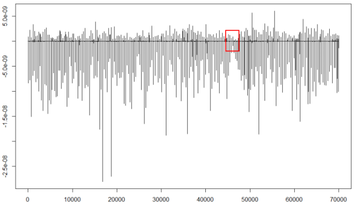
We should find the part containing the least negative minima (red square) and expand it to calculate the threshold:

plot(d25[46000:47000],type="l")

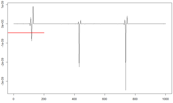
We can test the chosen threshold value to check if the signal is divided correctly:

fil<-filterecg(d25,-0.5e-9)
plot(fil,type="l")

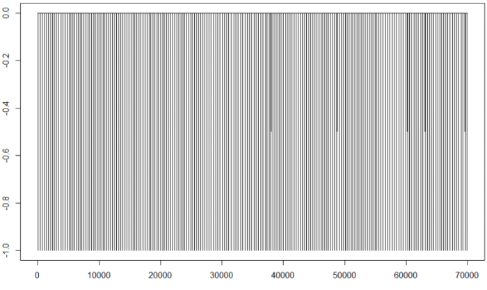
Now we only have points with values 0 or -1 (for the R points). If we do not observe anything strange, we can go on to calculate the intervals for the beats:

beats<-findr(signal,-0.5e-9)
plot(signal[beats[1,1]:beats[1,2]],type="l")

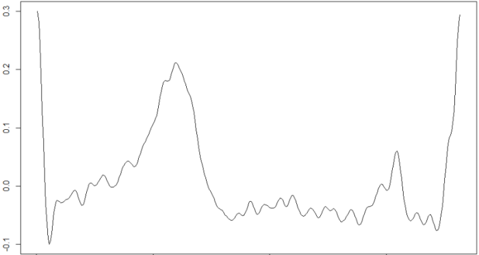
Where beats is an array in which each row is a beat, which starts at the position contained in the first column and ends at the position contained in the second. These data are then recorded in the files with .int extension associated to each .csv file with the ECG signal.

Calculating the RQA values

Once we can divide the electrocardiogram signal into beats, we have a basis to perform the RQA measurements with quite homogeneity. I am going to use as unit the signal between two consecutive R points, but this is an arbitrary criterion, you can use instead two or more beats as unit, or select a segment in such a way that the R point is inside it. This is one of the issues to decide, because the results obtained can vary a lot. In general, the more signal length we process, the longer the calculations will take, and the fewer samples we will have from the same signal recording. It may also be necessary to scale the data so that the range of values be equal for all the ECGs. I have chosen to scale all the ECGs in a range of values between -1.0 and 1.0.

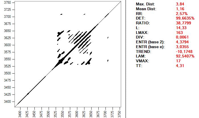
The selection of parameters includes the embedding dimension, the delay and the distance or radius, as I explained in the first article in this series. For the first two I have chosen the values 2 and 15. These values come from some studies that I have consulted, in which it is advised to extend the system to only two dimensions and using a delay of 0.03 seconds, which, with a sampling frequency of 500, corresponds to 15 points of the series. The distance or radius to consider two points as recurrent is calculated in each beat according to one of the RQA measurements, the proportion of recurrent points RR. The goal is to obtain a similar value for all beats, approximately 1.25. The reason is that this parameter is sometimes taken as a reference to calculate the optimal distance, since the results vary greatly depending on this radius. It is recommended to obtain values for the RR value that are not too high. This is a recurrence map of a heartbeat and the RQA values using a distance of 0.099:

And this is the same heartbeat, but using a distance of 0.2:

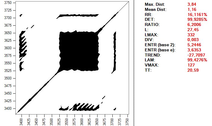
The important thing is to realize the complexity that can enclose simply to make a good choice of the parameters that we will use to perform the study. This process can take a long time and require many tests, in addition to a good level of knowledge about the subject and the tools used; it is not exactly a trivial procedure.

The code that performs the RQA calculations for an ECG segment is the mrqa function, which in turn uses the rqa function in the crqa package:

mrqa<-function(data,clsval,edim=3,sdel=1,rad,rr=0) {
tmprad<- rad;
repeat {
rqa<-crqa(data,
data,
delay=sdel,
embed=edim,
radius=tmprad,
normalize=0,
rescale=0,
mindiagline=2,
minvertline=2,
side="lower");
if (rr == 0) {
break;
}
if (rqa$RR-rr < -0.05) {
tmprad<-tmprad+0.0001;
}
else if (rqa$RR-rr > 0.05) {
tmprad<-tmprad-0.0001;
}
else {
break;
}
}
vrqa<-c(rqa$RR,rqa$DET,rqa$NRLINE,rqa$maxL,
rqa$L,rqa$ENTR,rqa$rENTR,rqa$LAM,rqa$TT,clsval);
return(vrqa);
}

For each beat, call this function to perform the recurrence analysis calculations. The result is a record with the RQA measures plus a numerical class identifier, used to train the neural networks. The data parameter contains the segment of the signal. clsval is the numeric identifier of the class assigned to the whole ECG. edim is the embedded dimension, sdel is the delay to use, rad is the distance or radius, and rr is an optional parameter to adjust the distance so that the RR measurement is as close as possible to it .If the value of the rr parameter is 0, no adjustment is made. Keep in mind that this feature can make calculations take much longer.

With the rqadata function, a complete ECG is processed:

rqadata<-function(vrqa,signalf,intf,clsval,edim=3,sdel=1,rad,
emin=-1,emax=1,rr=0) {
dint<-read.csv2(intf);
dsig<-read.csv2(signalf);
dnorm<-scaleecg(dsig[,1],emin,emax);
for(j in 1:length(dint[,1])) {
rqa<-mrqa(dnorm[dint[j,1]:dint[j,2]],clsval,edim,
sdel,rad,emin,emax,rr);
if (is.null(vrqa)) {
vrqa<-rqa;
}
else {
vrqa<-rbind(vrqa,rqa);
}
}
return(vrqa);
}

The vrqa parameter contains a dataframe with previous calculations to add new rows, or NULL to start a new data set. signalf contains the name of a csv file with the data of the ECG signal. intf is the file name with int extension associated with the ECG and containing the heartbeat indices. emin and emax are used to scale the values of the signal, and the rest of the other parameters are the same used in the previous mrqa function.

In the next article, we will train neural networks with the data obtained using this function.