Extending WinRQA II, series of recurrence measures

WinRQA is an application dedicated to recurrence plots, a tool that is used in the analysis of recurrence of complex time series. In this article I will introduce a new tool that I have added to the program. Until now, the measures of quantification of recurrence (RQM) were obtained only from a static portion of the original series. With the new tool, we can obtain a series of measures by moving a window along the entire original series and calculating the corresponding measurements to each of these windows.

For the technical details about this analysis type, I can recommend you this website entirely devoted to recurrent plots, or this book about recurrence quantification analysis.

In this link you can download the executables of the WinRQA application, and, in this another one, you can download the source code of the WinRQA project, written in CSharp with Visual Studio 2013. It is a Windows application, for the version 7 or later.

In this other link you can find the first article of the WinRQA application series.

Generate series to obtain recurrence measures

So that you can see what the new tool is for, let's first generate some example series. For this I will use the R program. If you want to bypass this part, in this link you can download the csv files with the generated series.

We will use the logistic function to generate the series. It is a very simple equation, with a single parameter and which is defined recursively:

X_n+1 = uX_n(1-X_n)

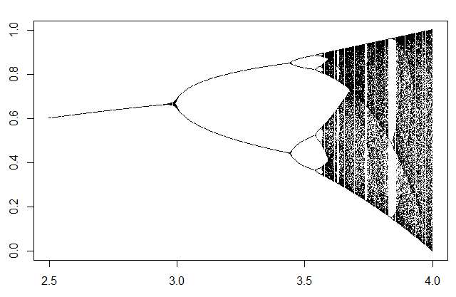
The parameter u can vary between 1 and 4, while x is always maintained in the interval (0, 1). This series presents different types of dynamics depending on the value of the parameter u, for values less than approximately 3.57, the series presents a stationary or periodic dynamics, but, from this value, the dynamics becomes chaotic, increasing the degree of chaoticity as we approach to 4, although with a small periodic area around 3.83.

This is a Feigenbaum diagram in which you can see how the number of different terms in the series varies according to the value of the parameter u:

This will allow us to generate a series with different dynamics. First, we will define a pair of auxiliary functions. You can create a script with them and save it in the working directory. I have named it dlogistic.R:

dfLog<-function(length, initial) { u<-3; du<-1/length; c<-1:(length); c[1] <- initial; for (i in 2:(length)) { v<-u*c[i-1]*(1-c[i-1]); c[i]<-v; u<-u+du; } return(c); } fLog<-function(u,length,initial) { c<-1:length; c[1]<-initial; for (i in 2:length) { c[i]<-u*c[i-1]*(1-c[i-1]); } return(c); }

The dfLog function generates a series of length values, with the provided initial value. The parameter u varies throughout the series from a value of 3 to an end value of 4, whereby the series goes through different types of dynamics. This generates a series of 2000 values, for example:

source("dlogistic.r") c<-dfLog(2000,0.5) plot(c,type="l")

Logistic time series with variable parameter

Then, save it in the dlog.csv file:

write.csv(c,"dlog.csv",row.names=F)

Before you can load it into the application, you have to remove the first row, with the name of the column.

You can generate another file with a series with only two different dynamics, using the fLog function. You have to pass to this function the parameter u with which you want to generate the series:

c<-fLog(3.78,1000,0.5) c<-c(c,fLog(3.98,1000,c[1000])) plot(c,type="l")

Which you can also save in a file (do not forget to delete the first row):

write.csv(c,"logistic2.csv",row.names=F)

Study of a time series with series of recurrence measures

With these two series generated, we can test the new tool I added to the WinRQA application. Let's open the dlog.csv file. In the toolbar is the RQMS button with which we can launch it. But, first, you have to set the Radius parameter to a value greater than or equal to zero (a good value for this series is 0.1), because with values less than zero no recurrence measures are calculated.

Once we launch the tool, a form with a toolbar like this appears:

The series has 2000 values. In the text boxes of the upper toolbar you can define the start and end point of the section of the series you are going to process, the step between point and point and the size of the window that the application have to use to construct each recurrence plot.

In the bottom toolbar, you can see all the measures of recurrence, with a white box on the right, and a button marked with a color palette that allows you to select a color for the graph of that measure. Only graphs of the measurements that have a color other than white will be drawn. When selecting the measures that you are going to add to the graph, it is necessary to take into account that the ranges of values can vary quite between each of them, reason why some graphs can appear like a straight line by effect of the difference of scales.

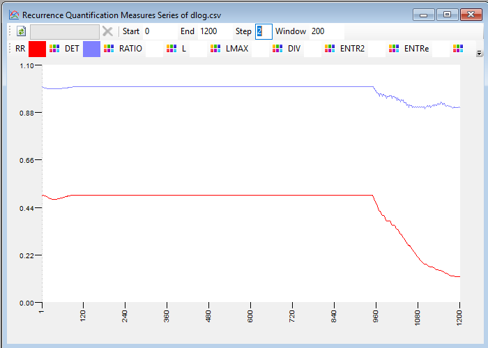
Once the measures are selected, you can launch the calculation with the first button in the upper toolbar. A graphic like this will be drawn:

Although the series changes from a periodic dynamics to a chaotic one approximately from position 1100, with this tool you can detect the change of dynamics well in advance, from position 950, approximately.

Although the periodic dynamics at the beginning of the series is variable, you can see that the measurements in that zone follow a straight line. The recurrence plot captures the type of dynamics, rather than other characteristics of the signal, such as its intensity or period.

Some of the measures are more appropriate than others to detect substantial changes in the series and their dynamics, or to characterize certain states with respect to others. With this you already have the basis to perform analysis of recurrence of time series.

Also be aware that this signal was generated artificially, so it doesn’t have noise. In general, signals from the real world have a certain amount of noise that often masks their characteristics, which is reflected in the values of the measures of recurrence. A good filter on the series, whenever possible, favors the accuracy of the analysis.

If you want to save a series of measures calculated by the program in a file, there is the Save CSV... option in the File menu (when this form is selected) with which you can save a file with the calculated measurements and the position of the series to which belongs to each of them. With this, you can perform an in-depth analysis of the data with a tool such as the R program.

This csv file has column names in the first row, the first column contains the position in the series, and the data is separated using the semicolon (;) character. The decimal places of the numbers are separated using the dot (.) character.

You can try with the other series, logistic2.csv, which has a smaller difference between the two zones with different dynamics. Keep in mind that the dynamics change from the 1000 position, going from chaotic to still more chaotic.