Extending WinRQA I, estimating delay and embedding dimension

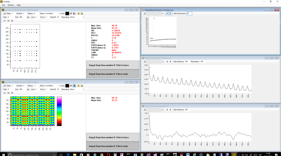
WinRQA is an application dedicated to recurrence plots, a tool that is used in the analysis of recurrence of complex time series. In this article I will present the first extension of the application, which mainly consists of a series of tool windows that will help you to make estimates on what may be the most appropriate delay to try to reconstruct the phase space of the system attractor and select the correct embedding dimension.

For the technical details about this analysis type, I can recommend you this website entirely devoted to recurrent plots, or this book about recurrence quantification analysis.

In this link you can download the executables of the WinRQA application, and, in this another one, you can download the source code of the WinRQA project, written in CSharp with Visual Studio 2013. It is a Windows application, for the version 7 or later.

In this other link you can find the first article of the WinRQA application series.

The features added in this new release of the application are the following:

• You can build recurrence plots of systems composed of more than one time series.
• You can create rectangular cross recurrence plots, between series with different dimensions.
• New tool to select the delay using the linear autocorrelation of the series.
• New tool to select the delay using the mutual information of the series.
• New tool to select the embedding dimension using the correlation dimension.

Recurrence plots of systems with more than one variable

Usually, the recurrence plots are used with series of values that we assume that form part of systems with more than one dimension. However, we can have theoretical models with more than one variable from which we have all the data. The program now allows you to read data composed of more than one time series, also in a csv file, with one column for each series, separated by the semicolon character (;).

These systems are treated as systems with fixed dimension, and you cannot modify the delay value or the embedding dimension, since you do not have to reconstruct any phase space, as you have the complete model. It can be used to make comparisons between this complete model and another simplified ones formed by a single series of values, for example.

In this link you can download sample data. The lorenz3D.csv file contains all the three series of a complete Lorenz system, while lorenzx.csv, lorenzy.csv and lorenzz.csv contain the time series corresponding to the variables X, Y and Z respectively. You can see that the series for X and Y are very similar, but different from Z, the whole system is best reproduced using two series, Z and X or Y, as shown by the joint recurrence plot, compared to the recurrence plot of the entire system.

Cross recurrence plots

In the initial version of the program, all recurrence plots were drawn as a square. However, cross recurrence plots can be rectangular, depending on the size of the windows of the series that we are crossing. In this new release I have included this feature, in addition to have corrected some inaccuracies in the construction of this type of plots.

Estimating the most appropriate delay

One of the fundamental parameters for correctly reconstructing the phase space is the delay to be used to build the additional dimensions from the original series. If you choose a too small delay, the reconstructed attractor will be too compressed, while excessively large delays produce highly deformed attractors due to the uncorrelation of the values of the series.

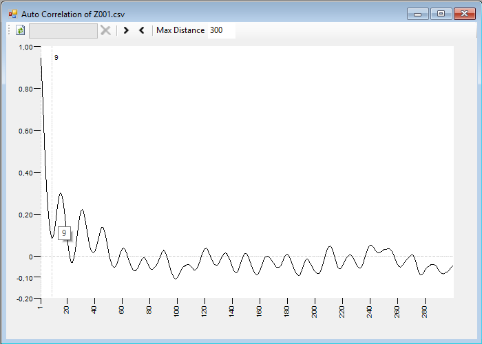
With the autocorrelation of the data in the series, you can detect linear relationships between segments separated by a certain period of time. To do this, simply calculate the linear correlation between the values of one segment of the series and another segment displaced a time t. We can draw a graph in which we represent in the vertical axis the correlation coefficient, which will take values between -1 and 1, and on the horizontal axis the different time intervals of separation between values.

You can indicate the maximum distance up to which you want to calculate the autocorrelation of the series. With the buttons you can limit the calculations to only those values between the beginning and / or end of the series window selected to build the current recurrence plot. The button is used to perform the calculations and draw the graph. These calculations are executed using a background process, so that you can continue using the application in case they take a long period of time.

By clicking the left mouse button on the graph, you can change the value of the delay in the recurrence plot main window. A very common criterion is to select the first local minimum of this graph as a reference delay.

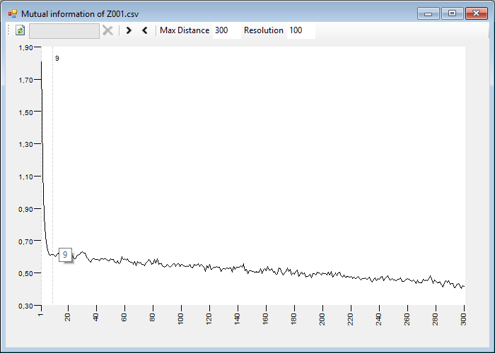
Another measure of autocorrelation that we can calculate is the mutual information. It is a generalization of the autocorrelation extended to the nonlinear relationships in the data. It is a probabilistic approach in which we use the conditional probability for pairs of values separated by a certain interval of time and the probability of each one of the values separately, according to the next formula:

P(s(t), s(t + τ))log2(P(s(t), s(t + τ))/P(s(t))P(s(t + τ)))

We calculate and add this value for all the terms of the complete series, or the selected window, and draw the graph as in the previous case.

In this window we can also indicate a value for the resolution that will be used to build the value histogram to calculate the probabilities. This value is the number of intervals in which we will divide the range of values of the series in order to discretize it.

As in the previous case, you can also use as a guide to select an appropriate value for the delay the first local minimum of this graph.

To use these tools, I have added a new toolbar to the main window:

The AC button will display the autocorrelation tool, and MI the mutual information tool.

Estimating the embedding dimension

In the new toolbar there is a last button, ED, which allows access a tool that can help you to estimate the most appropriate dimension to build the recurrence plot.

We know that, to properly reconstruct the phase space of the system while retaining its topological properties, we must use an embedding dimension with a value of at least 2d + 1, where d is the dimension of the system being studied.

On the other hand, the correlation dimension can be calculated as follows:

ν = lim(r->0) Log(C(r)) / Log(r)

Where r represents the radius we have selected for the recurrence plot and C(r) is the so called correlation integral, which is no more than the limit of the recurrence rate of the phase space reconstructed using that radius r to determine the neighborhood. It can be shown that this value constitutes a lower bound of the true dimension of the system.

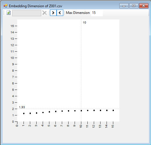
We can graph the value of this correlation dimension for different values of the embedding dimension, so that we can select the dimension as that from which notable changes in the correlation dimension no longer occur:

You can indicate the maximum dimension you want to explore. For each of the values of the dimension, on the horizontal axis, you can see the value of the correlation dimension, on the vertical axis, and a line for the nearest integer dimension above this value.

In this link you can find the source code parcially commented in CodeProject.

You can read about another extension of the application in the article extending WinRQA with series of recurrence measures.