Beyond chaos, randomness
In this article I will show how, through a very simple and totally deterministic process, we can move from a stationary system to a completely random one, going through periodic and chaotic dynamics. For this, I will generate several time series with these characteristics using the R program and several packages that can help us in the analysis of them.
In this link you can download the R source code that accompanies this article, with a series of auxiliary functions that I will use throughout it. First, you have to load this code:
source(“beyond-chaos.R”)
Two of the simplest functions and that allow us to generate the whole range of dynamics simply by varying a parameter are the logistic equation and the triangular application. These are recursive functions, where each term is obtained from the previous one. The first of them is expressed as follows:
Xn+1 = µXn(1 - Xn)
Where μ is a parameter that takes values in the interval (0, 4). The triangular application is written as follows:
Xn+1 = µ(1 – 2|0.5 - Xn|)
Here, the parameter μ takes values in the interval (0, 1).
With the R source code you can generate time series of the previous equations using the following functions:
fLog<-function(u,length,initial) {
    c<-1:(length+300);
    c[1] <- initial;
    for (i in 2:(length+300)) {
        c[i]<-u*c[i-1]*(1-c[i-1]);
    }
    return(c[-(1:300)]);
}
fTriangular<-function(u,length,initial) {
    c<-1:(length+300);
    c[1] <- initial;
    for (i in 2:(length+300)) {
        c[i]<-u*(1-2*abs(0.5-c[i-1]));
    }
    return(c[-(1:300)]);
}
Both have the same parameters, the length of the series that we want to get, the initial value of it and the value of the parameter μ. The first 300 values generated are discarded, because they can be transient values until the series stabilizes in its final dynamics, so that we get data without distortion.
To get an idea of the behavior of these two systems as we vary the parameter, we can draw a Feigenbaum diagram. It is a diagram in which in the abscissas axis we represent the different values of the parameter μ and, for each value of the parameter, we represent in the ordinates axis all the possible values that the series takes with the given parameter. In this way we can get an idea of the degree of complexity as we increase the value of the parameter, the zones with different dynamics and each critical point where bifurcations occur. To do this we use the following function (adapted from this article in R-bloggers):
feigenbaum<-function(start,end,step,fw) {
    pu<-seq(start,end,by=step);
    orbit<-sapply(pu,fw,initial=0.1,length=300);
    r<-sort(rep(pu,300));
    plot(r,orbit,pch=".");
}
For the logistic equation:
feigenbaum(2.5,4,0.003,fLog)
We obtain the following bifurcation diagram:
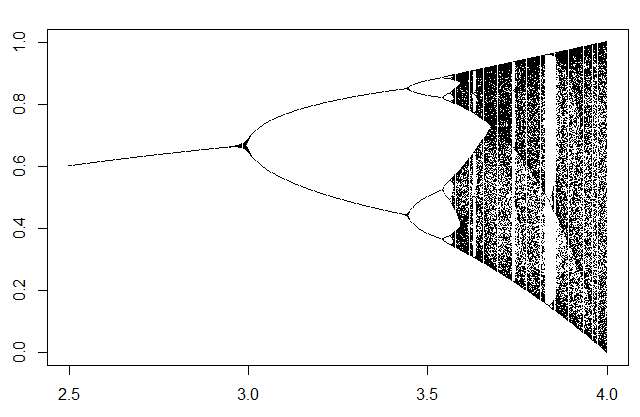
Where we can see that the dynamics is stationary until a μ value of 3, as the series only takes a single value, and from here they begin to produce bifurcations and the series goes doubling the number of values it takes, adopting a periodic dynamics, until reaching a point where the number of values becomes very large and we enter in the zone of chaotic dynamics, something beyond 3.5.
I will not go into details about the stationary and periodic dynamics, the only interest they have is that these equations generate time series with these dynamics in certain ranges of values of the μ parameter. Instead, the zone of chaotic dynamics presents interesting properties that we can study.
One of the main properties of chaotic systems is their sensitivity to initial conditions. This makes chaotic phenomena impossible to reproduce or, what is the same, to predict their evolution. Let's see an example using the triangular application, with a value of 0.95 for the μ parameter, in the chaotic zone, and an initial value of 0.1 compared to another of 0.1001:
plot(fTriangular(0.95,100,0.1),type="l")
lines(fTriangular(0.95,100,0.1001),col="red")
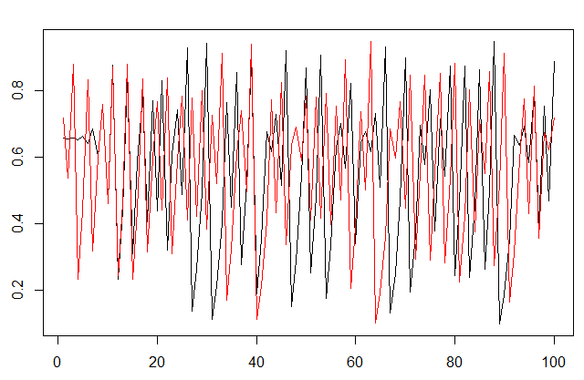
As you can see, the two series are totally different after a certain time, usually very short (in this case we have eliminated the first 300 terms of the series).
Of course, since it is a completely deterministic process, if we have the exact value of a term of the series, we can reproduce the series accurately from it, provided we use the same precision as in the original series, but in nature normally the measures we obtain are never exactly the same, so that chaotic phenomena are virtually irreproducible.
An interesting graphical tool to visually determine the degree of chaoticity of a system is the web diagram, which you can draw with the following functions:
fWebLog<-function(u,x) {
    return (u*x*(1-x));
}
fWebTriangular<-function(u,x) {
    return (u*(1-2*abs(0.5-x)));
}
webDiagram<-function(p, steps=500, fw) {
    xn<-seq(0,1,length.out=1000);
    xn1<-sapply(xn,fw,u=p);
    plot(xn,xn1,type='l',col="red");
    lines(xn,xn,lty=4);
    x0<-runif(1);
    xn<-x0;
    xn1<-0;
    for (i in 1:steps) {
        xf<-fw(p, x0);
        xn<-c(xn,x0);
        xn1<-c(xn1,xf);
        xn<-c(xn,xf);
        xn1<-c(xn1,xf);
        x0<-xf;
    }
    lines(xn,xn1);
}
The fWebLog and fWebTriangular functions are auxiliary functions for drawing the web diagram of the logistic equation or the triangular application. The function that draws the diagram is webDiagram, to which you have to pass the μ parameter (in p), the number of steps that we want to draw and the function you want to use to draw the diagram (fw).
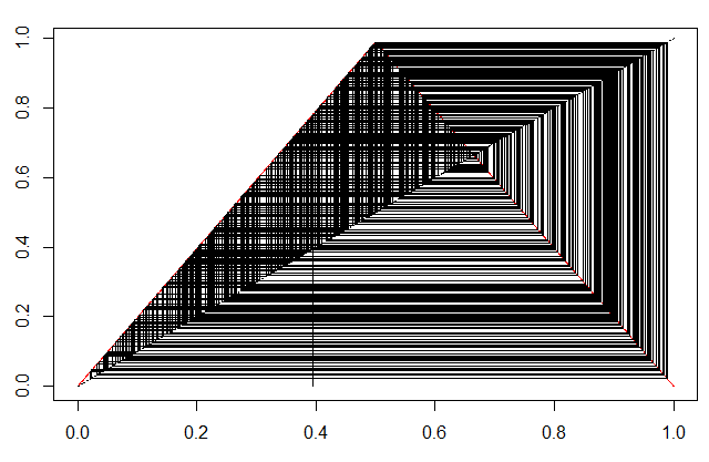
To draw this diagram, first we draw the curve of the function in the range of values that the given function takes (in our case it is always (0, 1)) and the diagonal line y = x. In the case of the logistic equation, the curve is a parabola, in the case of the triangular application, a triangle. Any value is taken to begin with, and a straight line is drawn from the abscissa axis until the curve, from this point, we draw a horizontal line until the y = x line and, from this point, we draw again a vertical line up to the curve. We repeat the process a certain number of times and we get something like this:
For the periodic zone of the logistic equation:
webDiagram(3.4,fw=fWebLog)
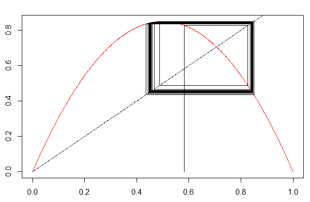
The dynamics are restricted to a well-defined area. However, in the chaotic zone, for example of the triangular application:
webDiagram(0.99,fw=fWebTriangular)
You can read more on these types of diagrams in this other article about web diagrams.
Although the time series is in principle unpredictable, we can verify its deterministic character using, for example, neural networks to try to approximate the function from a series of values. (In this link, you can find more about recurrent neural networks and time series). We will use Elman networks, for example with the RSNNS package:
require(RSNNS)
require(quantmod)
The first thing we will do is to construct an appropriate data set for its analysis with this type of networks, using the lagTS function:
lagTS<-function(ts,lags) {
    y<-as.zoo(ts);
    for (l in 1:lags) {
        y<-cbind(y,Lag(y,k=l));
    }
    return(na.omit(y));
}
In the dataframe that returns this function, we have a first column with the original series (ts), and a series of columns with values of the series displaced a determined number of terms (lags). Those last columns will be used to predict the values of the original time series. We generate the series and use, for example, 10 displaced series to predict:
tsl<-fLog(3.98,1000,0.2)
y<-lagTS(as.ts(tsl),10)
We use, by example, the first 900 values to train the network:
train<-1:900
inputs<-y[,2:11]
outputs<-y[,1]
fit<-elman(inputs[train],outputs[train],size=c(3,2),
    learnFuncParams=c(0.1),maxit=1000)
And we try to predict the rest of values:
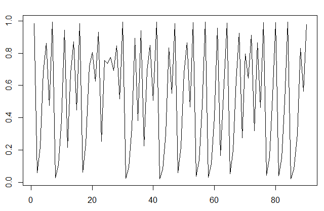
pred<-predict(fit,inputs[-train])
plot(as.vector(outputs[-train]),type="l")
lines(pred,col="red")
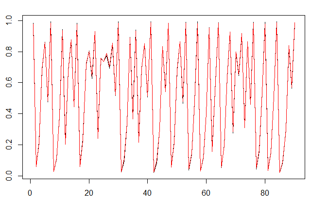
At least the next value of each term in the series is predicted with a very good approximation. If we try to predict more terms we will see that the actual and predicted data diverge quickly, but we can compare what happens if we do the same with data that, in principle, are not deterministic.
We could simply generate a series of random numbers with a function such as rnorm or runi. But the numbers generated by this type of functions are usually pseudorandom ones, also generated by deterministic processes, so we are going to use a truly random series (in fact, the results will not be very different, but this way we make sure). For this, there is this truly random numbers generator, which uses data from atmospheric noise instead of generating pseudorandom numbers.
In my case, I have generated a wav file with uniformly distributed white noise. To load a file of this type, you can use the audio package.
require(audio)
wv<-load.wave("soundfile.wav")
With this data, we can repeat the above procedure:
tsr<-(wv[1:1000] - min(wv[1:1000]))/(max(wv[1:1000])-min(wv[1:1000]))
y<-lagTS(as.ts(tsr),10)
inputs<-y[,2:11]
outputs<-y[,1]
fit<-elman(inputs[train],outputs[train],size=c(3,2),
    learnFuncParams=c(0.1),maxit=1000)
pred<-predict(fit,inputs[-train])
plot(as.vector(outputs[-train]),type="l")
lines(pred,col="red")
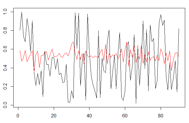
The values are normalized to take values between 0 and 1 because the network works better in this way, but we see that, in this case, the network has not been able to approximate the function that generates the series. Apparently there is a noticeable difference between the two sets of data in terms of their complexity, but, can we get these deterministic functions to become random?
In principle, with the logistic equation, we cannot use values greater than 4 for the μ parameter, since from this value the series becomes divergent. It seems that we must stop in a chaotic dynamics, but, according to the central limit theorem, if we add several variables with the same probability distribution, we will obtain another that will tend to have a normal distribution. We can try to average several of these deterministic series, initiated with different values so that we ensure they are all different, due to their sensitivity to the initial conditions. We will use the following function:
randFunc<-function(u1,u2,seed,length,count,fr) {
    v<-fr(u1,count,seed);
    x<-rep(0,length);
    for(i in 1:count) {
        x = x+fr(u2,length,v[i]);
    }
    return(x/count);
}
The initial values of the different series will be generated with another series with a value u1 for the parameter, we will generate count series of length values using the function fr, with the u2 parameter. The initial value for the series of initial values will be seed. The series generated will be averaged and the result of this operation will be returned.
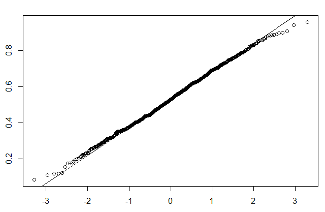
It may seem that we will need a lot of series to generate really random numbers, but let's see what happens if we average just 5 series:
r5<-randFunc(3.9,3.99,0.2,1000,5,fLog)
We can perform several tests of normality:
shapiro.test(r5)
W = 0.99781, p-value = 0.2119
qqnorm(r5)
qqline(r5)
We can even use recurrence plots to try to find traces of determinism in the generated pseudorandom data. We will use the crqa package to generate a recurrence plot for a chaotic series generated by the logistic equation (in this link you have more information on this subject, with the WinRQA application for recurrence plots):
Require(crqa)
tsl<-as.ts(fLog(3.98,198,0.2))
rqa<-crqa(tsl,tsl,delay=1,embed=1,rescale=0,radius=0.03,
    normalize=0,mindiagline=2,minvertline=2,side="both")
Since I have not found any function in the package to draw the recurrence plot, we can use this to do it:
recurrencePlot<-function(rp) {
    x<-rep(1:(dim(rp)[1]),dim(rp)[2])[as.vector(t(rp))==T];
    y<-as.vector(sapply(1:(dim(rp)[2]),
        rep,dim(rp)[1]))[as.vector(t(rp))==T];
    plot(x,y,pch=".",pty="s",asp=1);
}
The recurrence plot looks like that:
recurrencePlot(rqa$RP)
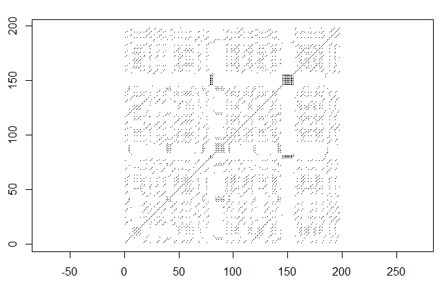
You can clearly see deterministic structures characterized by diagonal lines distributed fairly ordered in the graph. The DET RQA measure, or percentage of determinism, is quite high:
rqa$DET
68.86727
Now we can compare it with the recurrence plot of the truly random data obtained initially:
tsl<-as.ts(wv[1:200])
rqa<-crqa(tsl,tsl,delay=1,embed=1,rescale=0,radius=0.05,
    normalize=0,mindiagline=2,minvertline=2,side="both")
recurrencePlot(rqa$RP)
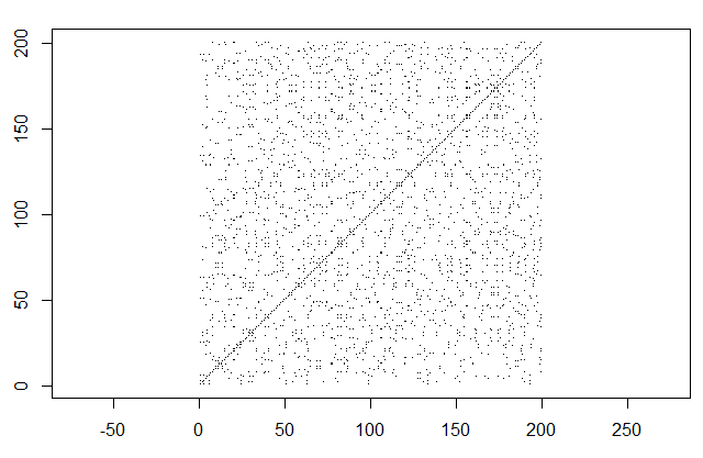
In this graph, deterministic structures are not observed, the points are isolated and the percentage of determinism is much lower:
rqa$DET
9.7621
And, what about the random series generated by averaging logistic series? we will also get its recurrence plot:
tsl<-as.ts(r5[1:200])
rqa<-crqa(tsl,tsl,delay=1,embed=1,rescale=0,radius=0.01,
    normalize=0,mindiagline=2,minvertline=2,side="both")
recurrencePlot(rqa$RP)
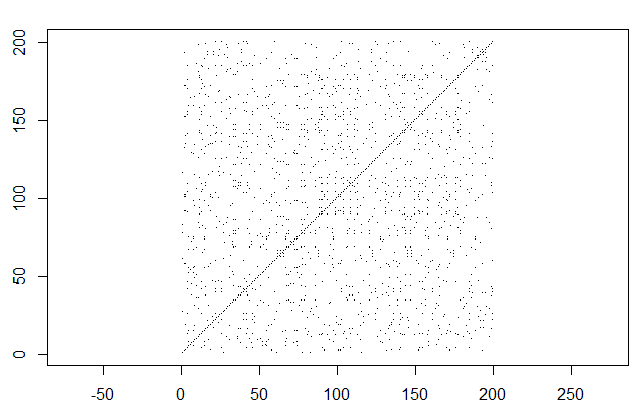
We can verify that it does not show traces of deterministic structures either. The rate of determinism is even better than in the case of truly random numbers:
rqa$DET
8.093995
With this we have verified how the randomness can arise from completely deterministic processes, so that it is indistinguishable from a real randomness, supposing that there really exists such a thing.
In any case, this procedure is not optimal to generate random numbers. If you are interested in this subject, you can read this article about normally distributed random number generation.


