Complex time series III, phase diagrams

In this new article in the series on graphic characterization of time series from a dynamic system with chaotic dynamics, I will talk about a way to represent such systems in the domain of space, independently of time, the phase diagram. With this type of diagram, you can see the attractors of the system. An attractor is a point, a curve, in general, a set of points to which converge the system equations, which gives us an idea of the typical behavior of that system.

If you want to start the series at the beginning, this is the link to the first article of the series on graphic characterization of complex time series. In this other link you can download the executable and source code of the GraphStudy project, written in CSharp with Visual Studio 2013.

So far I have used as an example the logistic equation, which has only one dimension. The one-dimensional attractors are not very interesting, since they are limited to a straight line, so, in this article I will use time series with more than one variable, generated by systems with two or three differential equations.

Let us begin with a simple attractor, with the following system of equations:

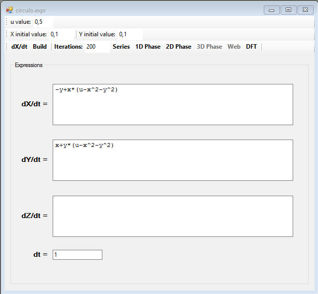
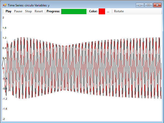
Periodic system of differential equations

The two series are linked together by the variables x and y, in this image there are two overlapping series, the red series is for the variable x and the black one for the variable y:

To view the attractor of the system, just press the 2D Phase button and, in the window that appears, the Play button to start the drawing. It is convenient to use a small value for dt, for example 0.001, and a large number of iterations, for example 10,000:

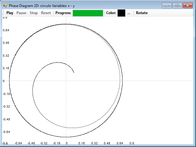
The drawing of the phase diagram is very easy, in every step we calculate the next term corresponding to each of the series, and then, we draw a point on the graph corresponding to those coordinates. This system begins in a point nearby to the origin (0.1, 0.1), and slowly follows a path until it ends confined in a circle. This circle is the attractor of the system, the trajectory until the circle is the transient state of the system, and the circle is what is called a limit cycle. This is clearly a periodic system.

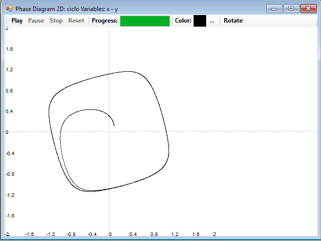
Another example of limit cycle can be seen in this other system of equations:

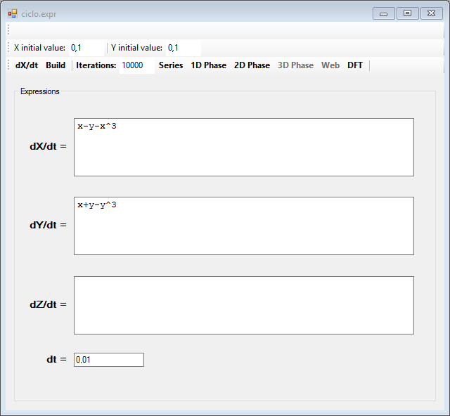
Another example of periodic system of equations — Another example of periodic system

And this is the limit cycle, which makes up its attractor:

Another examplo of limit cycle attractor — Another limit cycle attractor

Strange attractors

In the systems of equations that present a complex dynamics, the things are not so simple. These systems are characterized by complex attractors, with many paths, forming a fractal set of points, that is, a set whose dimension is a fractional number instead of an integer. These attractors are called strange attractors.

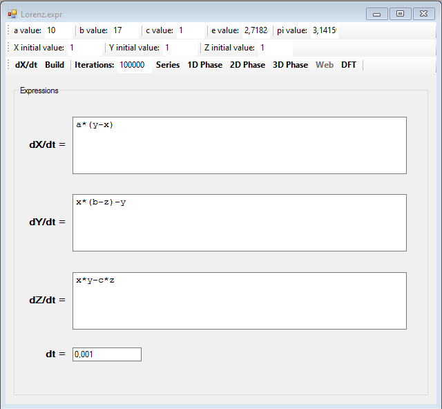
A classic example of a system having a strange attractor is the Lorentz model, which is a three-dimensional system with three differential equations:

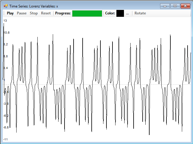
The series corresponding to the x and y coordinates are very similar; this is the series of x:

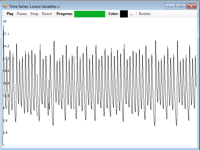
Time series for the xcoordinate in the Lorentz system — Time series for the x coordinate in the Lorentz system

And this is the one that corresponds to the z coordinate:

Time series for the z coordinate in the Lorentz system — Time series for the z axis in the Lorentz system

To draw the attractor of this system, press the 3D Phase button. The Lorenz attractor is obtained, with the known butterfly shape:

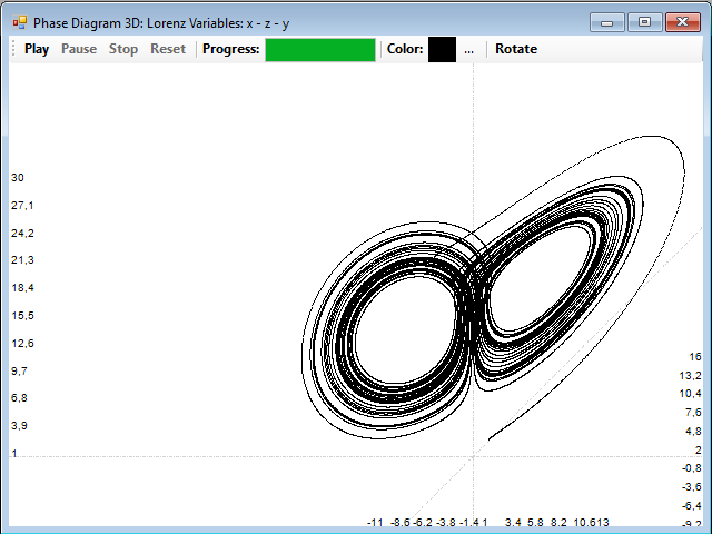
With the Rotate button you can vary the positions of the coordinate axes to see the attractor from different perspectives. This attractor presents typical characteristics of complex systems. Has a dimension somewhat greater than 2, it is estimated that between 2.05 and 2.07, with a fractal structure. It presents scale invariance, that is, as you expand an area in which there is a group of paths, always find one similar layout, with multiple paths too.

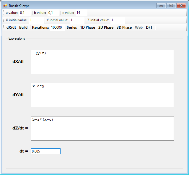
Another system with a strange attractor is the Rössler system, consisting of the following differential equations:

And this is the three-dimensional attractor of the system, the Rössler attractor:

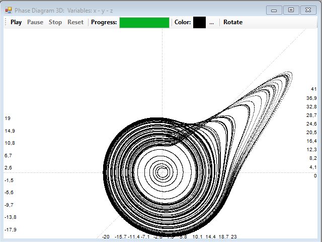
We say that these systems present deterministic chaos, because, although its dynamics is chaotic, they are generated by systems of fully deterministic equations.

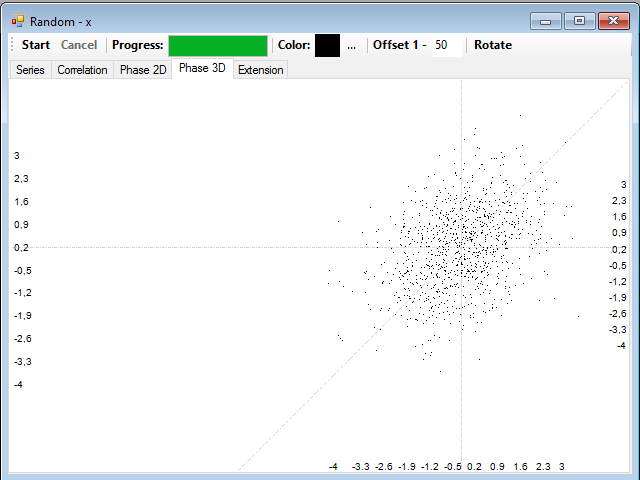
As you can see, it is easy to distinguish a periodic dynamics of a chaotic dynamics drawing the phase diagram for the series. If these are random and uncorrelated, what we will have is a shapeless cloud of points, like this:

In the next article of this series I will talk about the power spectrum and value distribution.