Complex time series I, basics

Many of the data sets with which we usually work are in the form of time series. A time series can be seen as the evolution of a dynamic system, characterized by some variables and parameters. Depending on the type of dynamic of the system, the series may be stationary, periodic, quasiperiodic, chaotic or random. In this series of articles, I will focus on the characterization of chaotic dynamics, which is presented by complex systems, by using graphical methods.

If you are unsure what these dynamical systems are, in this article you can see a brief introduction to complex systems.

Although to graphically study these complex models you can use any program that allows you to generate graphics and work with mathematical functions, such as R program, I developed a helper application to create graphics using a simple graphical user interface and with which you can export the generated series, or import them from R, so that we can work with them also with this application. In this link you can download the executable and source code of the GraphStudy project, written in CSharp with Visual Studio 2013.

The GraphStudy tool

To begin, let's see how to start working with the GraphStudy tool. It is an application with which you can write up to three equations and generate a series of graphs from them. The grammar of these expressions is based on that explained in the article design of the grammar for an expressions analyser. You can use the operators sum, difference, product, division, and exponentiation, and I added the sine (sin) and cosine (cos) functions. Also you can use the constants e and pi, to which are automatically given the corresponding value. You can use parentheses to change the precedence of operators.

To write a new system of equations, in the File menu select the New option:

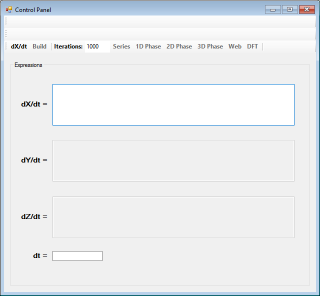
With the dX / dt button you can select if you want to write a system of differential equations or one with iterated functions:

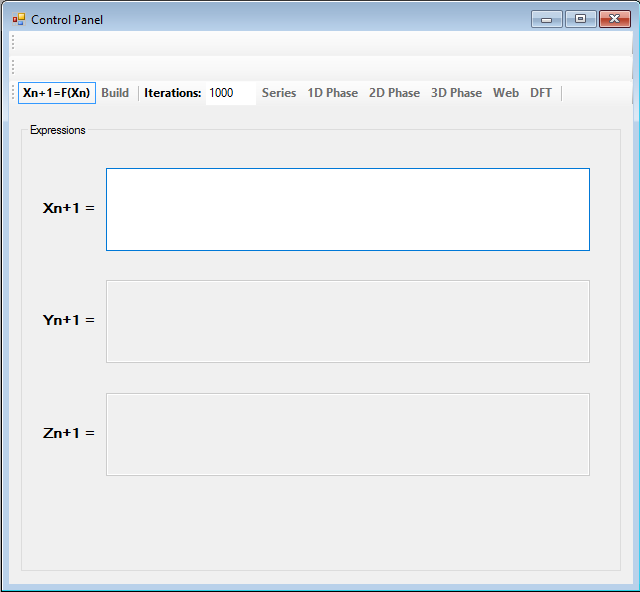
We can have up to three variables; X, Y and Z. Whenever write an equation for one of the variables, the box for editing the next is activated. Thus, we can have equations for X and Y, but not for Z and X.

Once written the equations, they must be compiled using the Build button. Done this, it will appear in the toolbars the constants and variables used in the equations, and you can give them values to generate the series. As variables can be used only X, Y and Z, as constants, you can use any other text string in unlimited number.

In the iterations text box you can define the number of terms of the series you want to generate. If you use differential equations, you have also to define the time step in the dt text box.

The logistic equation

One of the most common models to study the chaotic dynamics in time series is the logistic equation, which, in its reduced form, can be expressed as:

Xn+1 = µXn(1-Xn)

This simple equation is used in the study of population dynamics. The variable X takes values between 0 and 1. The key of this equation is in the μ parameter. Depending on its value, the series generated has a stationary, periodic or chaotic dynamics. The stationary dynamics is characterized by to tend to a single value. This equation has a stationary dynamic when μ is less than 3. From 3, the function becomes periodic. It begins oscillating between two values and, gradually, as increasing μ, the number of different values will double again and again, up to 3.57. From this value, the dynamics becomes chaotic, it appears sensitivity to initial conditions and the following values in the series begin to be unpredictable. In this link you can see an article to explore the logistic curve with R. With GraphStudy simply write the equation as an iterated function and click the Build button to compile:

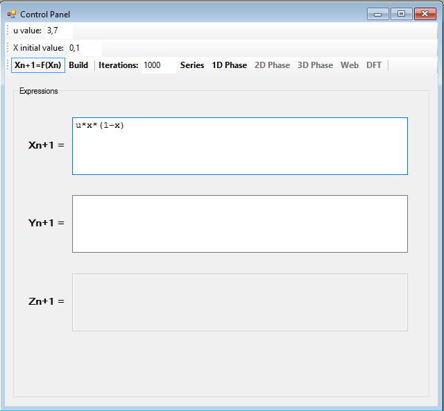
In the toolbar it appears the constant u, to which you have to give a value between 0 and 4, and the variable X, which you have to give an initial value in the range (0, 1).

Once you have defined and built a system of equations, in the File menu you can use the Save or Save as... options to save it to a file; and you can open it later using the Open... option.

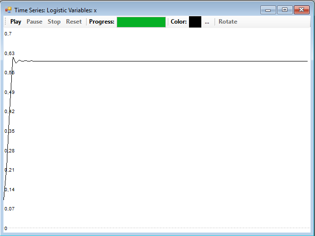
With the Series button you can generate the series corresponding to the selected parameters and initial values. For example, selecting a value for μ of 2.5, which belongs to the stationary domain of the series, and pressing the Play button on the window that appears when you press the Series button, you obtain the following graphic:

If you give to µ a value in the periodic zone, for example 3.2, you obtain a periodic series:

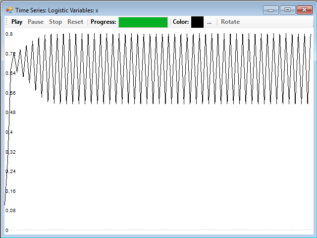
As an observation, look that there are a number of starting points in which the system is in an unstable situation until it reaches the final dynamics. Normally, in this series the N initial values are discarded to avoid having into account in the study these transient values, which are not characteristic of the series and can distort the results.

If you try with a value of μ in the chaotic zone, for example 3.7, you get the following result:

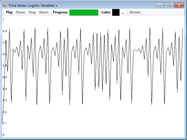
To check the sensitivity of the series to initial conditions, just open another window with the same equation and change the initial value of the variable X. generate the series, change the color of the graph in the window with the original series, by clicking on the button with the three points, and drag & drop the series generated with the new initial value on the window to superimpose them. In this example, you can see the difference between the series with an initial value of 0.1 and another one starting at 0.1001:

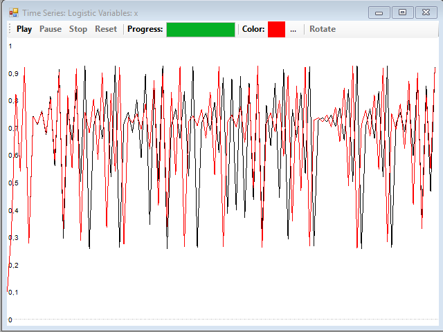
You can see that, at first, the two series match, but soon begin to take different values and diverged into two quite different series. We are in the presence of a complex dynamic.

The next article in the series is on using web diagrams to detect chaotic dynamics.